
Unsupervised monocular depth estimation with aggregating image features and wavelet SSIM (Structural SIMilarity) loss
 0
0Abstract
Unsupervised learning has shown to be effective for image depth prediction. However, the accuracy is restricted because of uncertain moving objects and the lack of other proper constraints. This paper focuses on how to improve the accuracy of depth prediction without increasing the computational burden of the depth network. Aggregated residual transformations are embedded in the depth network to extract high-dimensional image features. A more accurate mapping relationship between feature map and depth map can be built without bringing extra network computational burden. Additionally, the 2D discrete wavelet transform is applied to the structural similarity loss (SSIM) to reduce the photometric loss effectively, which can divide the entire image into various patches and obtain high-quality image information. Finally, the effectiveness of the proposed method is demonstrated. The training model can improve the performance of the depth network on the KITTI dataset and decrease the domain gap on the Make3D dataset.
Keywords
1. Introduction
Predicting depth from a single 2D image is a fundamental task in computer vision. It has been studied for many years with widespread applications in reality, such as visual navigation[1], object tracking[2,3], and surgery[4]. Moreover, accurate depth information is vital with considerable influence on the performance of autonomous driving, where expensive laser sensors are usually used. Recent advances in convolutional neural networks (CNNs) show their powerful ability to learn an image’s high-dimensional features. Especially, the mapping relationship between image feature and image depth can be built. Generally, monocular depth estimation approaches can be classified into three categories: supervised[5–9], semi-supervised[10], and unsupervised[11–19]. Both supervised and semi-supervised learning rely on the image depth ground truth. Using a laser sensor to obtain the depth ground truth of many images is expensive and difficult. However, unsupervised learning has the advantage of eliminating the dependency on the depth ground truth. Therefore, more and more studies are training monocular depth estimation networks using unsupervised methods from monocular images or stereo pairs. Compared with stereo pairs, a monocular dataset is more general as the input of network. However, it needs to estimate the pose transformation between consecutive frames simultaneously. As a result, a pose estimation network is necessary that outputs relative 6-DoF pose with given sequences of frames as input.
Most unsupervised depth estimation networks[5,8,11] are constructed using typical CNN structures. On the one hand, a series of max-pooling and stride operations may reduce the network’s ability to learn image features and cause lower quality of depth map. On the other hand, to improve the performance of the network, deeper convolution layers are designed in depth CNNs. They increase the computational burden of the network and bring extra hardware cost. In most cases, the cost of the network overweighs the benefits generated by the network. To improve the depth estimation performance without increasing the network burden, an end-to-end unsupervised monocular depth network framework is proposed in this paper. Inspired by previous work[20] on the image classification task, aggregated residual transformations (ResNeXt) are migrated to the depth estimation field. Based on typical depth CNNs, the ResNeXt block is embedded to extract more delicate image features in the encoder network. In addition, more accurate mapping relationship between the feature map and depth map can be built without bringing extra network burden. In addition, the accuracy of depth network suffers from some noise (e.g., haze and rain) in the complex images. To reduce the influence of noise, the 2D wavelet discrete transform[21] is applied to SSIM loss, which can recover high-quality clear images. A sample of depth prediction is shown in Figure 1.
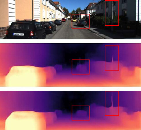
Figure 1. The input image from the KITTI dataset (top); the baseline MonoDepth2[22] (M, ResNet50, without pre-training) depth prediction; (middle) and our result (bottom).
In summary, our proposed network can improve depth prediction accuracy without increasing network computational complexity. The contributions of this paper can be summarized as follows:
Based on a ResNeXt block, a novel feature extraction module for depth network is developed to improve the accuracy of depth prediction. It can not only extract high-dimensional image features but also guide the network to more deeply learn the scene to get farther pixel depth.
A wavelet SSIM loss is applied to photometric loss to converge the training network. Various patches with clearer image information computed by DWT are used as input, rather than the whole image, to the loss function, which can remove some noise (daze, rain, etc.) from the image.
The rest of this paper is organized as follows. The related work on depth estimation is discussed in Section 2. Section 3 presents an overview of the proposed network architecture and the loss function. Then, some experiments based on different datasets are presented to verify the performance of the proposed network in Section 4. Finally, the conclusions and future work are introduced in Section 5.
2. Related work
2.1. Supervised depth estimation
Based on vast training datasets with depth ground truth, depth estimation networks show great performance in recent years. Eigen et al.[5] first demonstrated the huge potential of CNNs in depth prediction from a single image. They obtained reliable depth estimation results by using a coarse-to-fine depth network. Further, Liu et al.[7] combined CNNs with Markov random fields (MRF) to learn intermediate features, acquiring clearer local details of depth map in the visual effect. Laina etal.[8] changed the structure of the depth network and proposed a residual CNNs to model the mapping relationship between monocular image and its corresponding depth map. Instead of using absolute depth ground truth, Chen et al.[9] acquired relative depth value labels between the random pixel pairs from the image to train the depth network. In addition, to obtain dense depth map, Kuznietsov et al.[10] proposed a semi-supervised method which used both sparse ground truth depth for supervised learning and a photo consistent loss in stereo images for unsupervised learning.
Even though the works mentioned above significantly contributed to depth estimation, these methods still suffer from the limitation of depth ground truth.
2.2. Unsupervised depth estimation
Based on stereo or monocular images, unsupervised learning methods focus on how to design the supervisory signal. The typical solution is to use view synthesis as a proxy task[11,12,14–24], so as to get rid of depth ground truth.
2.2.1. Unsupervised depth estimation from stereo images
Using stereo images is a feasible unsupervised way to train a monocular depth network. A depth network can be obtained by predicting the left–right pixel disparities between stereo pairs during training. It can be applied when predicting monocular image depth. Garg et al.[11] first used stereo pairs to train depth network with known disparities between left and right images and acquired great performance. Inspired by the authors of[11], Godard et al.[12] designed a novel loss function which enforced both left-right and right–left disparities consistency produced from stereo images[12]. Zhan et al.[13] extended the stereo-based network architecture by increasing the visual odometry network (VO). The performance of Zhan’s network was superior to other unsupervised methods at that time. To recover absolute scale depth map from stereo pairs, Li et al.[14] proposed a visual odometry system (UnDeepVO), which was capable of estimating the 6-DoF camera pose and recovering the absolute depth value.
2.2.2. Unsupervised depth estimation from monocular images
For monocular depth estimation, it is necessary to design an extra pose network to obtain pose transformation between consecutive frames. Both depth and pose networks are trained together with loss function. Zhou et al.[16] pioneered the training of depth networks with monocular video. They proposed two separate networks (SfMLearner) to learn image depth and inter-frame pose transformation. However, the accuracy of the depth network was often limited by the influence of moving objects and occlusion. Their work motivated some researchers to consider these shortcomings. Subsequently, Casser et al.[17] developed a separate network (struct2depth) to learn each moving object motion, but their work was based on the condition that the number of moving objects needed to be hypothesized in advance. In addition, researchers found that the optical flow method could be employed to deal with moving object motion. Yin et al.[18] developed a cascading network framework (GeoNet) to adaptively learn rigid and non-rigid object motion. Recently, multi-task training methods have been proposed. Luo et al.[19] intended to train depth, camera pose, and optical flow networks (EPC++) jointly with 3D holistic understanding. Similarly, Ranjan et al.[24] proposed a competitive collaboration mechanism (CC) with depth, camera motion, optical flow, and motion segmentation together. Both Luo and Ranjan’s joint network inevitably increased the difficulty of the training network and the computational burden of the network.
From the above works, we can see that most studies aim to improve the accuracy of the depth network by changing the network structure or building robust supervisory signal. It is worth noting that these methods bring network complexity and computational burden while improving the network accuracy. This motivates us to study how to balance both sides. Poggi et al.[15] presented an effective pyramid feature extraction network, which can be implemented in real-time on CPU. However, the accuracy of the network cannot satisfy the requirements of practical applications. Xie et al.[20] provided a template with aggregated residual transformations (ResNeXt), which achieved a better classification result without increasing network computation. Because of the advantages of ResNeXt, we apply it to the image depth prediction field. The ResNeXt block serves as a feature extraction module of the depth network to learn the image’s high-dimensional features. The proposed approach is not only independent of depth ground truth, but also does not increase computational burden.
3. Method
The proposed method contains two parts: an end-to-end network framework and a loss function. The network framework consists of a depth network and a pose network, as shown in Figure 2. Given unlabeled monocular sequences, the depth network outputs the predicted depth map, while the pose network outputs the 6-DoF relative pose transformation between adjacent frames. The loss function is made up of the basic photometric loss and the depth smoothness loss, and it couples both networks into the end-to-end network.
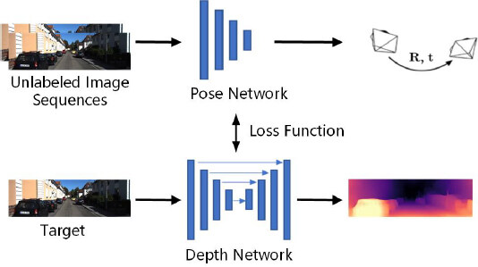
Figure 2. The overall architecture of both the depth network and the pose network.
3.1. Problem statement
The aim of the unsupervised monocular depth network is to develop a mapping relationship Γ : I(p) → D (p), where I(p) is an arbitrary image, D(p) is the predicted depth map of the image I(p), and p is per pixel in the image I(p). Establishing a more accurate mapping function Γ is considered in this paper, which includes: (a) a simple and effective network pipeline without increasing network computational complexity; and (b) a high-quality depth map D(p) with subtle details for a given input image I(p).
For Item (a), our focus is to change the basic building blocks of the depth CNN structure using aggregated residual transformations (ResNeXt). In the depth network, ResNeXt serves as feature extraction module to learn the image’s high-dimensional features without increasing network computational burden. For Item (b), low-texture regions in the low-scale depth map are weakened, bringing inaccurate image reconstruction. Inspired by the authors of[22], four images with full resolution are reconstructed instead of building four images with different resolutions. Before the four images are reconstructed, the predicted four-scale depth map needs to be resized to the same resolution as input image with bilinear interpolation.
A single image I(p) is considered as the input of the depth network. The designed depth network outputs five-scale feature map Fk×(k ∈ 1, 2, 3, 4, 5) in the encoder network and four-scale depth map Dn in the decoder network. The mapping function is designed as
where m denotes the number of feature maps, m = 5. n represents the scale factor of depth map, n ∈ 0, 1, 2 ,3. k denotes the resolution of feature map Fk× is 1/2k of the input resolution.
Then, bilinear interpolation is applied to each predicted depth map Dn× to acquire the full-resolution depth map R(I(p)), which is defined as follows:
where U represents bilinear interpolation which recovers the resolution 1/2n of Dn× to the input full resolution.
The full-resolution depth map R(I(p)) is necessary to reconstruct the input image. Given two adjacent images with a target view and a source view 〈It(p), Is(p)〉, and the predicted 6-DoF pose transformation T, a pixel in the target image pt’s mapping homogeneous coordinate ps→t in the source image Is is computed as
where K is camera intrinsic matrix, pt is set as the normalized coordinate in target image It, and Tt→s is a 4 × 4 matrix transformed by T.
Therefore, the reconstructed target image
3.2. Feature extraction module
Equation (1) is applied to exploit higher-dimensional features and acquire feature map Fk× with more details. Since the ResNeXt block has a great performance on classification task. the feature extraction module is constructed by the ResNeXt block. In contrast to the ResNet used in most depth CNNs, the ResNeXt block aggregates more image features without bringing more network parameters, as shown in Figure 3.
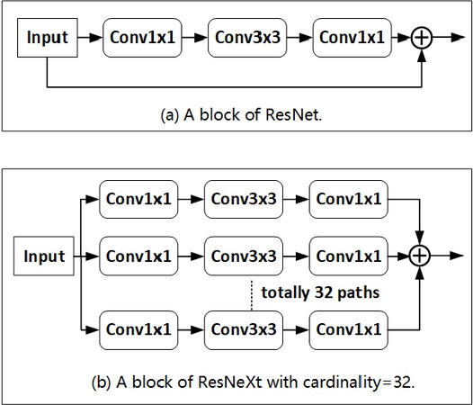
Figure 3. The architecture of ResNet and ResNeXt block: (a) the ResNet block; and (b) the aggregated residual transformations. Both have similar complexity, but the ResNeXt block has better adaptability and expansibility.
The ResNeXt block puts the input image into 32 parallel groups and learns the image features, respectively. Each group shares the same super-parameters and is designed as a bottleneck structure which cascades three convolution layers with the kernel sizes, respectively, being 1 × 1, 3 × 3, and 1 × 1. The first 1 × 1 convolution layer extracts high-dimensional abstract features by reducing (or increasing) output channels. Given an input image I with H×W×C′ resolution, the transformation function Ti of the ;th group maps image I to the high-dimensional feature map Ti(I). The aggregated output f(I) is the summation of the output of all the groups, which is defined as follows:
where C is the number of groups, C = 32, with C as cardinality.
Then, to be closely connected with the input, a residual operation is used, F(I). The aggregated output feature map for each module is
3.3. Network architecture
The proposed depth estimation network employs U-Net structure including an encoder network and a decoder network. The encoder network is built by embedding the ResNeXt block[20]. It transforms the three-dimensional monocular image into multi-channel feature map. The decoder network builds the relationship between extracted feature map and the depth map by a series of upsample and convolution (Up-convolution) operations, as shown in Figure 4.
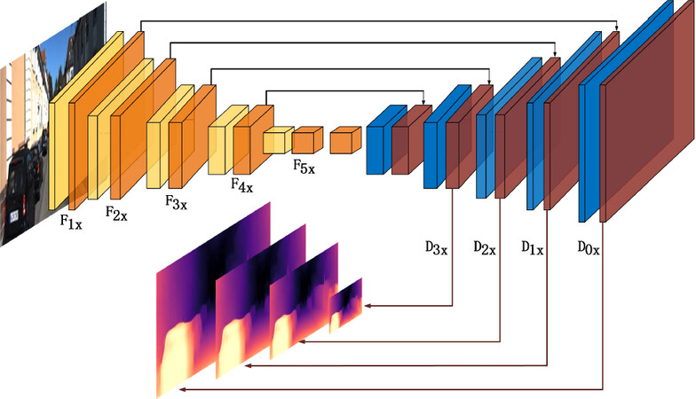
Figure 4. The proposed depth network architecture. The width and height of every cube indicates output channels, and the size is reduced by half every time. The first yellow cube is a convolution block, while the rest of the yellow cubes are ResNeXt blocks. The orange blocks represent the five-scale feature map, Fk×. In the decoder network, convolution layers are blue. Upsample and convolution operations are red. Dn× is the four-scale depth map.
(1) To eliminate texture copy artifacts in the depth map, the Up-convolution operation[22] instead of deconvolution is used to reshape the feature map. (2) Due to max-pooling and stride operations ignoring some local features and causing some details to be lost in the depth image, skip connections are used to merge the corresponding feature maps for encoder network into decoder network and obtain fine image details. (3) Inspired by the authors of[22], we resize all depth maps to the same resolution as input using bilinear interpolation (represented by the U operation in Equation (2)).
The structure for the pose network is designed as a standard ResNet18 encoder, which is similar to the one in[22]. More input images in the pose network bring more accurate depth estimation under certain conditions. However, to reduce the number of training parameters of pose network, the pose network has N (N = 3) adjacent images as input. Therefore, the shape for convolutional weights in the first layer is (3 × N) × 64 × 3 × 3 rather than the default 3 × 64 × 3 × 3 in the pose network The output of the pose network has 6 * (N – 1) channels. In addition, our pose network is trained without pre-training. All convolution layers are activated by ReLU function[25] except for the last layer. When the pose result is evaluated, an image pair is fed into pose network to produce six output channels, the first three-channel is rotation, and the last three-channel is translation.
3.4. Wavelet SSIM loss
In general, the SSIM[26] loss is included in the photometric loss to measure the degree of similarity between images. In this paper, the 2D discrete wavelet transform (DWT) is applied to SSIM to decrease the photometric loss. Firstly, The DWT divides an image into some patches with different frequencies. Then, the SSIM of each patch is computed. To preserve high-frequency image details and avoid producing “holes” or artifacts in some low-texture regions, it can flexibly adjust the weights of each patch of SSIM loss.
In the 2D discrete wavelet transform (DWT), low-pass and high-pass filters are performed on an image to obtain the convolution results. For instance, four filters, fLL,fLH, fHL, and fHH, are obtained by the low-pass filter multiplying the high-pass filter. The DWT divides an image into four small patches with different frequencies through these four filters, which can remove unnecessary interference from the images (e.g., haze and rain). Iteratively the DWT can be formulated as follows:
where i is the iterative time of DWT.
To preserve high-frequency image details and avoid producing image artifacts, a coarse-to-fine manner is adopted to change the image resolution in the SSIM loss. The DWT divides the image into four patches:
The ratios of the four patches are
where ri is the weight of each patch. The initial value of r is 0.7. t is the target image, s is the source image.
Initially, before the DWT divides the image, the SSIM loss between the target image and source image is calculated. The total wavelet SSIM (LWSSIM) loss is
3.5. Total loss function
There are two main parts in the loss function: the target image photometric loss LP is calculated by reconstructing the target image, while the smoothness loss LS of depth image compels the predicted depth map to be smooth, given the input target image It and its reconstructed image
In general, the image photometric loss contains the structural similarity metric (SSIM)[26] and the regularization loss ζ1. The wavelet SSIM loss is used to replace SSIM loss in photometric loss. Therefore, the image photometric loss is defined as
where we empirically set α = 0.85.
When computing the photometric loss from different source images, most previous approaches average the photometric loss together into every available source images. However, the second assumption requests that each pixel in the target image is also visible to the source image. However, this assumption is easily broken. It is inevitable that some moving objects and occlusions exist in the scene; thus, some pixels are available in one image but are not available in the next image. As a result, inaccurate pixel reconstruction and the photometric error are caused. Following the work in[22], the minimum photometric loss at each pixel in the target image is computed instead of the average photometric loss. Note that this method can only correct the photometric loss but not eliminate it. Therefore, the final per-pixel photometric loss is
In addition, the performance of depth network suffers from the influence of moving objects in the image. These moving pixels should not be involved in computing the photometric loss. Therefore, a binary per-pixel mask μ in[22] is applied to automatically recognize moving pixels (μ = 0) and static pixels (μ = 1). The mask μ only includes some pixels whose photometric error of the reconstructed image
[ ] is the Iverson bracket. The auto-masking photometric loss[22] is
The second-order gradients of the depth map are used to make the depth map smooth. Because the edge or corner in the depth map should be less smooth than other flat regions, the gradient of the depth map should be locally smooth rather than fully smooth. Therefore, a Laplacian[23] is applied to automatically perceive the position of each pixel. Different from the method in[23], it is used at every scale instead of a specific scale. The Laplacian template is second-order differencing with four neighborhoods. It can reinforce object edges and weaken the region of slowly varying intensity. The smoothness loss of this pixel receives a lower weight when the Laplacian is higher. The smoothness loss is defined as follows:
where ∇ is the Laplacian operator.
Therefore, the total loss function is
The final total loss is averaged per pixel, batch, and scale.
4. Experiments
To evaluate the effectiveness of our approach, some qualitative and quantitative results are provided about depth and pose prediction. KITTI dataset is the main data source to train and test depth networks. The KITTI odometry split was used to train and test our pose network. Meanwhile, the Make3D dataset was used to evaluate the adaptive ability and generalization of the proposed network.
4.1. Implementation details
The proposed depth network has dense skip connections which can fully learn deep abstract features. The network was trained from scratch without pre-training model weights and post-processing. The Sigmoid output of depth map is D = 1/(ασ + β), where σ and β make the depth value D between 0.1 and 100 units. In our experiments, the MonoDepth2[22] was set to standard ResNet50 encoder for monocular depth network, ResNet18 for pose network, and without pre-training. Here, we simplify its name to MD2 for the rest of the paper.
Deep learning framework PyTorch[27] was used to implement our model. For comparison, the KITTI dataset was resized and downsampled to 640×192. The proposed network used Adam[28] optimizer with β1 = 0.9 and β1 = 0.999 to train 22 epochs. The batch size was set as 4 and the smoothness term γ was set to be 0.001. The learning rate was set to be 10–4 for the first 20 epochs and reduced by a factor of 10 for the remaining epochs. The settings for the pose network were the same as in[22]. In addition, a single NVIDIA GeForce TITAN X with 12 GB GPU memory was used in our experiments.
4.2. Evaluation metrics
To evaluate our method, we used some standard evaluation metrics, as shown in Table 1.
The standard evaluation metrics for network
| Abs Re | |
| Sq Re | |
| RMSE | |
| RMSElog | |
| δ |
|I| is the number of pixels in image I.
4.3. KITTI eigen split
The KITTI Eigen split[16] was used to train the proposed network. Before the network was trained, Zhou’s[16] preprocessing was used to remove static images. As a result, the training dataset had 39,810 monocular triplets, which contain 29 different scenes. The validation dataset had 4424 images, and there were 697 testing images. The image depth ground truth of the KITTI dataset was captured by Velodyne laser. Following the work in[22], the intrinsics of all images were same, the principal point of the camera was set as image center, and the focal length was defined as the average of all focal lengths in the KITTI dataset. In addition, the depth predicted results were obtained by using the per-image median ground truth scaling proposed in[16]. When the results were evaluated, the maximum depth value was set to be 80 m and the minimum to be 0.1 m.
Figure 5 shows some visual examples of predicted depth maps. Our proposed model in the last row generates higher quality depth maps and gets clearer object edges than the other models. Some quantitative results are also provided in Table 2. The evaluation metrics are defined in Table 1. For the first four indices, lower scores are better. For the last three indices, higher scores are better. In Table 2, all results are shown without postprocessing[21]. The last row is the predicted result of our proposed method. The accuracy of depth prediction is improved when compared with other methods trained on monocular images. It is demonstrated that the proposed method is effective. Generally, the fewer input images in the pose network have a negative impact on the accuracy of the depth network. Even though only three frames are used to train the pose network at a time, our depth prediction results still outperform the other methods. Note that, some methods in Table 2[18,19,24] were trained with multiple tasks.
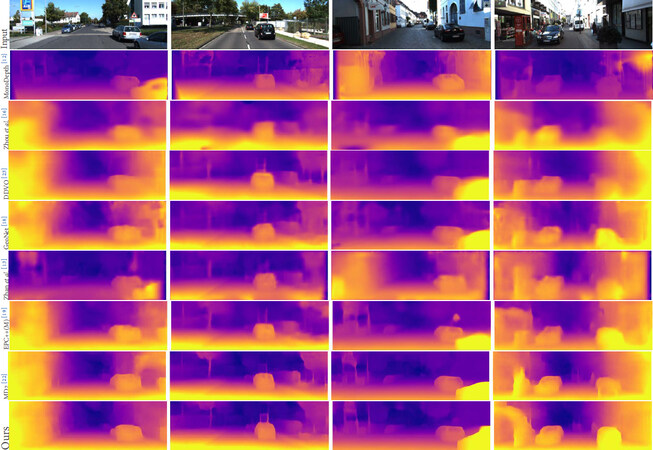
Figure 5. Qualitative results on the KITTI Eigen split. The results are compared with some existing unsupervised methods.
The quantitative results. This table shows the results of our method and other existing methods on KITTI Eigen split[16]. The best results in every category are in bold. M denotes the training dataset is monocular. * represents the newer results from GitHub
| Lower is better | Higher is better | |||||||
|---|---|---|---|---|---|---|---|---|
| Method | Train | AbsRel | SqRel | RMSE | logRMSE | δ < 1.25 | δ < 1.252 | δ < 1.253 |
| Zhou*[16] | M | 0.183 | 1.595 | 6.709 | 0.270 | 0.734 | 0.902 | 0.959 |
| Yang[29] | M | 0.182 | 1.481 | 6.501 | 0.267 | 0.725 | 0.906 | 0.963 |
| Mahjourian[30] | M | 0.163 | 1.240 | 6.220 | 0.250 | 0.762 | 0.916 | 0.968 |
| GeoNet*[18] | M | 0.149 | 1.060 | 5.567 | 0.226 | 0.796 | 0.935 | 0.975 |
| DDVO[23] | M | 0.151 | 1.257 | 5.583 | 0.228 | 0.810 | 0.936 | 0.974 |
| DF-Net[31] | M | 0.150 | 1.124 | 5.507 | 0.223 | 0.806 | 0.933 | 0.973 |
| LEGO[32] | M | 0.162 | 1.352 | 6.276 | 0.252 | - | - | - |
| Ranjan[24] | M | 0.148 | 1.149 | 5.464 | 0.226 | 0.815 | 0.935 | 0.973 |
| EPC++[19] | M | 0.141 | 1.029 | 5.350 | 0.216 | 0.816 | 0.941 | 0.976 |
| Struct2depth[17] | M | 0.141 | 1.026 | 5.291 | 0.215 | 0.816 | 0.945 | 0.979 |
| MD2[22] | M | 0.131 | 1.023 | 5.064 | 0.206 | 0.849 | 0.951 | 0.979 |
| Ours | M | 0.125 | 0.992 | 5.076 | 0.203 | 0.858 | 0.953 | 0.979 |
4.4. Additional study
4.4.1. Make3D dataset
The collected scene of the Make3D dataset is different from the KITTI dataset. Therefore, the Make3D dataset is often used to evaluate the adaptability of a network model. Our depth model trained on the KITTI dataset was tested on the Make3D dataset to evaluate its adaptability. The qualitative results are shown in Figure 6. The second column is the depth ground truth. Compared with MD2[22], the visual results of our model can get the global scene information and capture more object details. It can be seen that our method is useful and has great scene adaptability.
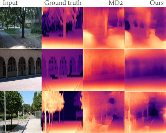
Figure 6. Some predicted depth examples on the Make3D dataset. The models were all trained on KITTI only, monocular, and directly tested on Make3D.
4.4.2. Validating proposed ResNeXt and LWSSIM
Table 3 shows the result of depth prediction for different components of the proposed method. “Basic” is the MD2 mentioned above. The results clearly prove that the contributions of our proposed terms to the overall performance. It is evident that discrete wavelet transform (DWT) can recover a high-quality clear image and improve the accuracy of depth prediction. The accuracy of depth prediction for both single-scale and multiscale supervisions are shown. Compared with the multi-scale method, the result of the single-scale method is better. The reason for this phenomenon is hypothesized to be that the low-resolution image has over-smoothed pixel color, which can easily cause inaccurate photometric loss.
Ablation studies on ResNeXt and LWSSIM
| Lower is better | Higher is better | |||||||
|---|---|---|---|---|---|---|---|---|
| Method | Train | AbsRel | SqRel | RMSE | logRMSE | δ < 1.25 | δ < 1.252 | δ < 1.253 |
| Basic[22] | M | 0.131 | 1.023 | 5.064 | 0.206 | 0.849 | 0.951 | 0.979 |
| Basic+ ResNeXt | M | 0.127 | 0.990 | 5.109 | 0.205 | 0.854 | 0.950 | 0.978 |
| Basic+ResNeXt+LWSSIM | M | 0.125 | 0.992 | 5.076 | 0.203 | 0.858 | 0.953 | 0.979 |
| Basic+ResNeXt+LWSSIM (single scale) | M | 0.123 | 0.980 | 4.987 | 0.200 | 0.862 | 0.954 | 0.979 |
4.4.3. Network capacity
To show our proposed network can improve accuracy without increasing network capacity, the number of network parameters and the floating-point operations per second (FLOPs) for the network were computed to evaluate the capacity of the proposed network. The quantitative results are shown in Table 4. For the sake of fair comparison, the pose network of MD2 and ours were set as ResNet50. Note that ResNet50 serves as our pose network only for comparison. The pose network adopted in the proposed overall framework is still ResNet18. Compared with MD2, our proposed method improves the accuracy of the depth network without adding extra computational burden, as expected.
Model capacity, params is the number of parameters of depth network, totalparas indicates the total parameters for both depth and pose network, and M is million unit.
| Method | Params | FLOPs | Total params |
|---|---|---|---|
| MD2(ResNet50)[22]: | 25.56M | 1.0×10¹⁰ | 61.8M |
| ours | 25.03M | 1.0×10¹⁰ | 61.3M |
4.5. Pose estimation
Our pose model was evaluated on the standard KITTI odometry split[16]. This dataset includes 11 driving sequences. Sequences 00–08 were used to train our pose network without using pose ground truth, while Sequences 09 and 10 were used to evaluate our pose model. The average absolute trajectory error with standard deviation (in meters) was used as evaluation metric. Godard’s[22] handling strategy was followed to evaluate the result of the two-frame model on the five-frame snippets. Because Godard’s[22] pose estimation results (M, ResNet50 for depth network, and ResNet18 for pose network) are not provided, we retrained and obtained the trained result (MD2).
Only two adjacent frames were taken in our pose model at a time, as shown in Table 5. The output was the relative 6-DoF pose between images. Even though our pose network structure is the same as that in MD2, our pose model obtains better performance than MD2. In addition, the results are comparable to other previous methods. Thus, it is observed that the proposed depth network has a positive effect on pose network.
Odometry results on the KITTI odometry dataset
| Method | Sequence09 | Sequence10 | Frames |
|---|---|---|---|
| ORB-SLAM[33] | 0.014 ± 0.008 | 0.012 ± 0.011 | - |
| DDVO[26] | 0.045 ± 0.108 | 0.033 ± 0.074 | 3 |
| Zhou*[16] | 0.05 ± 0.039 | 0.034 ± 0.028 | 5→2 |
| Mahjourian[30] | 0.013 ± 0.010 | 0.012 ± 0.011 | 3 |
| GeoNet[18] | 0.012 ± 0.007 | 0.012 ± 0.009 | 5 |
| EPC++(M)[19] | 0.013 ± 0.007 | 0.012 ± 0.008 | 3 |
| Ranjan[24] | 0.012 ± 0.007 | 0.012 ± 0.008 | 5 |
| MD2(M) | 0.018 ± 0.009 | 0.015 ± 0.010 | 2 |
| ours | 0.017 ± 0.010 | 0.015 ± 0.010 | 2 |
5. Conclusions
A versatile end-to-end unsupervised learning framework of monocular depth and pose estimation is developed and evaluated on a dataset in this paper. Aggregated residual transformations (ResNeXt) are embedded in depth network to extract the input image’s high-dimensional features. In addition, the proposed wavelet SSIM loss is based on 2D discrete wavelet transform (DWT). Different patches with different frequencies are computed by DWT as the input to the SSIM loss to converge the network, which can recover high-quality clear image patches. The evaluation results show that the performance of depth prediction is improved while the computational burden is reduced. In addition, the proposed method has great adaptive ability on the Make3D dataset and can decrease the domain gap between different datasets. In future work, how to further optimize the whole system will be considered.
Declarations
Authors’ contributions
Made substantial contributions to conception and design of the study and performed data analysis, data acquisition and interpretation: Li B Provided administrative, technical guidance and material support: Zhang H, Wang Z, Hu L
Availability of data and materials
Not applicable.
Financial support and sponsorship
This work is supported by the National Key R&D Program of China (2018YFB1305003), National Natural Science Foundation of China(61922063), and Shanghai Shuguang Project (18SG18).
Conflicts of interest
All authors declared that there are no conflicts of interest.
Ethical approval and consent to participate
Not applicable.
Consent for publication
Not applicable.
Copyright
© The Author(s) 2021.
REFERENCES
1. Zhang K, Chen J, Li Y, Zhang X. Visual tracking and depth estimation of mobile robots without desired velocity information. IEEE Trans Cybern 2018;50:361-73.
2. Xiao J, Stolkin R, Gao Y, Leonardis A. Robust fusion of color and depth data for RGB-D target tracking using adaptive range-invariant depth models and spatio-temporal consistency constraints. IEEE Trans Cybern 2017;48:2485-99.
3. Gedik OS, Alatan AA. 3-D rigid body tracking using vision and depth sensors. IEEE Trans Cybern 2013;43:1395-405.
4. van der Sommen F, Zinger S, With P, et al. Accurate biopsy-needle depth estimation in limited-angle tomography using multi-view geometry. In: Medical Imaging 2016: Image-Guided Procedures, Robotic Interventions, and Modeling. vol. 9786. International Society for Optics and Photonics 2016. p. 97860D.
5. Eigen D, Puhrsch C, Fergus R. Depth map prediction from a single image using a multi-scale deep network. arXiv preprint arXiv: 14062283 2014.
6. Chang Y, Jung C, Sun J. Joint reflection removal and depth estimation from a single image. IEEE Trans Cybern 2020; doi: 10.1109/TCYB.2019.2959381.
7. Liu F, Shen C, Lin G. Deep convolutional neural fields for depth estimation from a single image. In: Proceedings of the IEEE Conference on Computer Vision and Pattern Recognition 2015. pp. 5162-70.
8. Laina I, Rupprecht C, Belagiannis V, Tombari F, Navab N. Deeper depth prediction with fully convolutional residual networks. In: 2016 Fourth International Conference on 3D Vision (3DV). IEEE; 2016. pp. 239-48.
9. Chen W, Fu Z, Yang D, Deng J. Single-image depth perception in the wild. Advances in Neural Information Processing Systems 2016;29:730-38.
10. Kuznietsov Y, Stuckler J, Leibe B. Semi-supervised deep learning for monocular depth map prediction. In: Proceedings of the IEEE Conference on Computer Vision and Pattern Recognition 2017. pp. 6647-55.
11. Garg R, Bg VK, Carneiro G, Reid I. Unsupervised cnn for single view depth estimation: Geometry to the rescue. In: European Conference on Computer Vsion. Springer; 2016. pp. 740-56.
12. Godard C, Mac Aodha O, Brostow GJ. Unsupervised monocular depth estimation with left-right consistency. In: Proceedings of the IEEE Conference on Computer Vision and Pattern Recognition 2017. pp. 270-79.
13. Zhan H, Garg R, Weerasekera CS, et al. Unsupervised learning of monocular depth estimation and visual odometry with deep feature reconstruction. In: Proceedings of the IEEE Conference on Computer Vision and Pattern Recognition 2018. pp. 340-49.
14. Li R, Wang S, Long Z, Gu D. Undeepvo: Monocular visual odometry through unsupervised deep learning. In: 2018 IEEE International Conference on Robotics and Automation (ICRA). IEEE; 2018. pp. 7286-91.
15. Poggi M, Aleotti F, Tosi F, Mattoccia S. Towards real-time unsupervised monocular depth estimation on cpu. In: 2018 IEEE/RSJ International Conference on Intelligent Robots and Systems (IROS). IEEE; 2018. pp. 5848-54.
16. Zhou T, Brown M, Snavely N, Lowe DG. Unsupervised learning of depth and ego-motion from video. In: Proceedings of the IEEE Conference on Computer Vision and Pattern Recognition 2017. pp. 1851-58.
17. Casser V, Pirk S, Mahjourian R, Angelova A. Depth prediction without the sensors: Leveraging structure for unsupervised learning from monocular videos. In: Proceedings of the AAAI Conference on Artificial Intelligence. 2019. pp. 8001-8.
18. Yin Z, Shi J. Geonet: Unsupervised learning of dense depth, optical flow and camera pose. In: Proceedings of the IEEE Conference on Computer Vision and Pattern Recognition 2018. pp. 1983-92.
19. Luo C, Yang Z, Wang P, et al. Every pixel counts++: Joint learning of geometry and motion with 3d holistic understanding. IEEE Trans Pattern Anal Mach Intell 2019;42:2624-41.
20. Xie S, Girshick R, Dollár P, Tu Z, He K. Aggregated residual transformations for deep neural networks. In: Proceedings of the IEEE Conference on Computer Vision and Pattern Recognition 2017. pp. 1492-500.
21. Yang HH, Yang CHH, Tsai YCJ. Y-net: Multi-scale feature aggregation network with wavelet structure similarity loss function for single image dehazing. In: ICASSP 2020-2020 IEEE International Conference on Acoustics, Speech and Signal Processing (ICASSP). IEEE; 2020. pp. 2628-32.
22. Godard C, Mac Aodha O, Firman M, Brostow GJ. Digging into self-supervised monocular depth estimation. In: Proceedings of the IEEE/CVF International Conference on Computer Vision 2019. pp. 3828-38.
23. Wang C, Buenaposada JM, Zhu R, Lucey S. Learning depth from monocular videos using direct methods. In: Proceedings of the IEEE Conference on Computer Vision and Pattern Recognition 2018. pp. 2022-30.
24. Ranjan A, Jampani V, Balles L, et al. Competitive collaboration: joint unsupervised learning of depth, camera motion, optical flow and motion segmentation. In: Proceedings of the IEEE/CVF Conference on Computer Vision and Pattern Recognition 2019. pp. 12240-49.
26. Wang Z, Bovik AC, Sheikh HR, Simoncelli EP. Image quality assessment: from error visibility to structural similarity. IEEE Trans Image Process 2004;13:600-612.
27. Ketkar N. Introduction to pytorch. In: Deep learning with python. Springer; 2017. pp. 195-208.
28. Kingma DP, Ba J. Adam: a method for stochastic optimization. arXiv preprint arXiv:14126980 2014.
29. Yang Z, Wang P, Xu W, Zhao L, Nevatia R. Unsupervised learning of geometry with edge-aware depth-normal consistency. arXiv preprint arXiv:171103665 2017.
30. Mahjourian R, Wicke M, Angelova A. Unsupervised learning of depth and ego-motion from monocular video using 3d geometric constraints. In: Proceedings of the IEEE Conference on Computer Vision and Pattern Recognition 2018. pp. 5667-75.
31. Zou Y, Luo Z, Huang JB. Df-net: Unsupervised joint learning of depth and flow using cross-task consistency. In: Proceedings of the European Conference on Computer Vision (ECCV) 2018. pp. 36-53.
32. Yang Z, Wang P, Wang Y, Xu W, Nevatia R. Lego: Learning edge with geometry all at once by watching videos. In: Proceedings of the IEEE Conference on Computer Vision and Pattern Recognition 2018. pp. 225-34.
Cite This Article
Export citation file: BibTeX | RIS
OAE Style
Li B, Zhang H, Wang Z, Liu C, Yan H, Hu L. Unsupervised monocular depth estimation with aggregating image features and wavelet SSIM (Structural SIMilarity) loss. Intell Robot 2021;1(1):84-98. http://dx.doi.org/10.20517/ir.2021.06
AMA Style
Li B, Zhang H, Wang Z, Liu C, Yan H, Hu L. Unsupervised monocular depth estimation with aggregating image features and wavelet SSIM (Structural SIMilarity) loss. Intelligence & Robotics. 2021; 1(1): 84-98. http://dx.doi.org/10.20517/ir.2021.06
Chicago/Turabian Style
Li, Bingen, Hao Zhang, Zhuping Wang, Chun Liu, Huaicheng Yan, Lingling Hu. 2021. "Unsupervised monocular depth estimation with aggregating image features and wavelet SSIM (Structural SIMilarity) loss" Intelligence & Robotics. 1, no.1: 84-98. http://dx.doi.org/10.20517/ir.2021.06
ACS Style
Li, B.; Zhang H.; Wang Z.; Liu C.; Yan H.; Hu L. Unsupervised monocular depth estimation with aggregating image features and wavelet SSIM (Structural SIMilarity) loss. Intell. Robot. 2021, 1, 84-98. http://dx.doi.org/10.20517/ir.2021.06
About This Article
Copyright

Data & Comments
Data
0

 Cite This Article 29 clicks

 Like This Article 31
likes
Like This Article 31
likes


Comments
Comments must be written in English. Spam, offensive content, impersonation, and private information will not be permitted. If any comment is reported and identified as inappropriate content by OAE staff, the comment will be removed without notice. If you have any queries or need any help, please contact us at support@oaepublish.com.