
On the elastodynamics of a five-axis lightweight anthropomorphic robotic arm


Abstract
This paper presents elastodynamic modeling and analysis for a five-axis lightweight robotic arm. Natural frequencies are derived and visualized within the dexterous workspace to show the overall performances and compare them to the frequencies when the robotics is with payload. The comparison shows that the payload has a relatively small influence to the first- and second-order frequencies. Sensitivity analysis is conducted, and the system's frequency is more sensitive to the second joint stiffness than the others. Moreover, observations from the displacement response analysis reveal that the robotics produces linear elastic displacements of the same level between the loaded and unloaded working modes but larger rotational deflections under the loaded working condition. The main contribution of this work lies in that a systematic approach of elastodynamic analysis for serial robotic manipulators is formulated, where the arm gravity and external load are taken into account to investigate the dynamic behaviors of the robotic arms, i.e., frequencies, sensitivity analysis, and displacement responses, under the loaded mode.
Keywords
1. Introduction
Lightweight robotic arms and anthropomorphic assistive robots with high payload capacity are desired for applications of industry and welfare, among other fields, such as assisted daily living [1-3], pick-and-place operations [4], etc. Pick-and-place robots are well suited for a static environment where the task is repeated and precise tolerances are demanded[5]. As a mechanical system, the dynamic characteristics of the robotic arm is of importance to account for the requirements of application, such as high precision, speed, and payload. Henceforth, higher natural frequencies and low elastic displacements of a robotic manipulator will allow higher operational speeds and working cycles for efficient productivity[6]. Natural frequencies indicate the condition in which a mechanism tends to vibrate[7,8]. Differing from a structure or element, the dynamic behavior of a mechanism usually heavily depends on its architecture and configurations[9]; thus, it is not a trivial task to characterize the robot dynamics throughout the workspace, which calls for the kineto-elastodynamic analysis to provide the fundamentals of the modeling, design and control.
The elastodynamic modeling and analysis of a robotic manipulator have been reported previously[10,11], and they are roughly grouped into two categories: lumped modeling[12-15] and distributed-flexibilities modeling[9,16-19]. In general, with lumped modeling it is simpler to model the elastodynamic equation with acceptable computational accuracy, while the latter provides a more accurate model but with the high-dimensional generalized coordinate space and more complex procedure[20]. The commonly used method to study the elasticity of the robotic manipulators is the virtual joint method (VJM) as it can provide acceptable computation accuracy that is close to that of finite element analysis (FEA)[21]. Besides, VJM can be time efficient. VJM is based on pseudo-rigid body models with "virtual joints"[22-25]. Generally, the link flexibilities and linear/torsional springs take into account the bending contributions to the mechanism [26-29]. The stiffness formulated in the above approaches is limited to a subspace defined by the degrees of freedom (dofs) of the manipulator end-effector. Pashkevich et al.[30] overcame this issue by introducing a full-mobility lumped-parameter model by localizing 6-dof virtual springs to the links' ends and/or joints. In these models, the stiffness matrix is calculated in an unloaded equilibrium configuration of a robotic manipulator. On the other hand, the external loads directly influence the manipulator equilibrium configuration and, consequently, may modify the static properties. The lightweight design of the robotics accordingly decreases the link structural stiffness; thus, the robot geometry change due to external loads should be considered[31-33]. Consequently, elastodynamics of the robotic manipulators is an important concern in their design and applications. Based on the matrix structural analysis, Cammarata et al.[9,34] proposed an algorithm to assemble the stiffness matrix to investigate the manipulators with lower kinematic pairs. In this manner, the overall robotic manipulator in-parallel architecture can be split into substructures for modeling the elastodynamics[35]. Wu et al.[36] analyzed and compared the stiffness and natural frequencies of a 3-dof parallel manipulator with/without a redundant leg, where the joint deformations are ignored in the stiffness modeling. The small-amplitude deformations of the active joints can be considered as parameter uncertainties in terms of small variations to be integrated into the dynamic model[37]. Briot and Khalil[14] used the Newton-Euler recursive approach to develop a general symbolic elastodynamic calculation model for flexible parallel robots. Taghvaeipour et al.[15] derived the posture-dependent stiffness matrix in the elastodynamic modeling by resorting to the generalized spring concept. The previous models were established in the nominal configurations; hence, the geometry changes of the manipulator in this work are considered in the elastodynamic modeling and analysis.
In this paper, the elastodynamic characteristics of a lightweight robotic arm are investigated. The arm gravity and external load are taken into account to derive the stiffness matrix. Isocontours of natural frequencies over the dexterous workspace are formulated and sensitivity analysis is conducted. The frequencies and displacement responses of the robotics with payload are analyzed and compared with the dynamic behaviors of the unloaded mode. The main contribution of this work lies in that a systematic approach of elastodynamic analysis for serial robotic manipulators is formulated, where the arm gravity and external load are taken into account to investigate the dynamic behaviors of the robotic arms, i.e., frequencies, sensitivity analysis, and displacement responses, under the loaded mode.
2. Kinematics of the lightweight robotic arm
The lightweight robotic arm under study has five degrees of freedom (dof)[38], which adopts a modular design approach, as shown in Figure 1. The revolute joints are composed of CPU series gearboxes of Harmonic Drive and Maxon motor with gearhead to enhance the torque capabilities, except Joint 4 with geared motor. The actuators of joints are controlled by Maxon EPOS controllers. The Controller Area Network (CANopen) bus is adopted to build the communications between motors and controllers, and A CAN–USB interface is used to establish the communications between CANopen bus and the PC[38]. In accordance with the Denavit-Hartenberg (D-H) convention[39], the Cartesian coordinate systems are established accordingly.
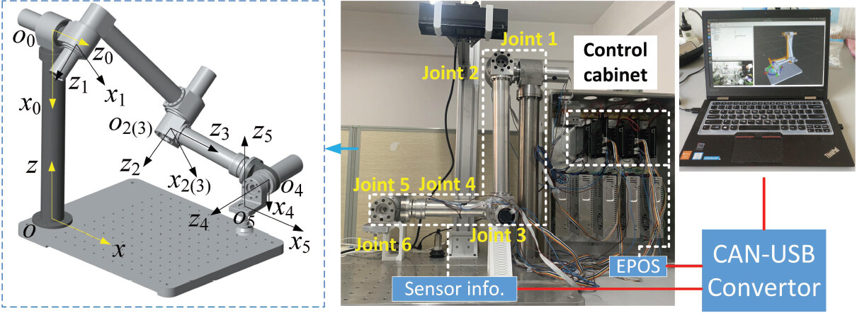
Figure 1. The 5-dof lightweight robotic arm and its coordinate systems[38].
2.1. Kinematics of robotic arm
Throughout this work, i, j, and k stand for the unit vectors of the x-axis, y-axis, and z-axis, respectively. The transformation matrix in forward kinematics of the end-effector in reference frame is expressed as
with
where D-H parameters are given in Table 1, and the inverse geometry problem for this robotics is well documented in the literature [8].
D-H parameters of the 5-dof robotic arm
| Joint i | αi | ai[mm] | di[mm] | θi |
|---|---|---|---|---|
| 1 | π/2 | 0 | 250 | θ1 |
| 2 | 0 | 600 | 0 | θ2 |
| 3 | π/2 | 0 | 0 | θ3 |
| 4 | –π/2 | 0 | 600 | θ4 |
| 5 | π/2 | 0 | 150 | θ5 |
2.2. Kinematic jacobian matrix
The velocities between the joints and end-effector are mapped with the Kinematic Jacobian matrix
where
with
where Ri–1 and qi–1 denote the rotation matrix and position vector of the transformation matrix from the reference coordinate system to the (i – 1)th coordinate system, respectively, which can be extracted from
2.3. Dexterous workspace
The reachable workspace of the robotic arm can be visualized by considering the limitation of the joint displacements and link dimensions. To effectively perform the kinematic performance, a dexterous workspace is defined, throughout which the inverse of the condition number of the Jacobian matrix is greater than 0.2, namely κ–1 (J) ≥ 0.2. Since the Jacobian matrix of Equation (4) is not homogeneous, a characteristic length[41] is introduced to normalize the Jacobian matrix as follows:
By constraining the condition number of the kinematic Jacobian matrix, a regular dexterous workspace is quarterly visualized in Figure 2.
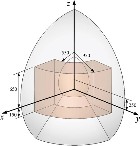
Figure 2. The quarter of the reachable and dexterous workspace (red volume) for the robotic arm.
3. Elastodynamic model of robot
The elastodynamic modeling procedure pertains to the calculation of the stiffness and mass matrices of the manipulator, which is described in the following sections. Prior to the derivation of the elastodynamic model, the following assumptions are made:
The actuator stiffness is considered as an 1-dof torsional spring, while the link is considered as cantilever with a 6-dof spatial spring located at the end but treated as rigid.
The centers of mass of the regular components are coincident with their geometric centers.
The sum of moments of inertia of the actuators and Harmonic drivers are considered as lumped.
3.1. Stiffness matrix
To derive the elastodynamic equation of the robotic arm, the stiffness matrix is calculated with the virtual spring approach[42], based on the screw coordinates[43]. Hence, the component masses and external loads are taken into account to compute the Cartesian stiffness matrix. Figure 3 shows the VJM model of the robotic arm, where Gj, j = 1, 2, ..., 7, stands for the gravity and F for the external loads.
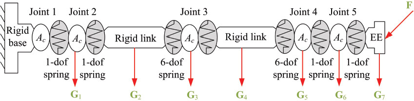
Figure 3. Virtual spring model of the 5-dof robotic arm with auxiliary loads, where Ac stands for the actuator and EE for end-effector.
Let θ and θ' be the original and the deformed displacements of the virtual springs, respectively, following the principle of virtual work, i.e. the work of the auxiliary forces is equal to the work of internal forces τθ, namely,
where the virtual displacements δtj and δt can be computed from the linearized geometrical model derived from δtj =Jj(θ' – θ) and δt =Jθ(θ' – θ), respectively, Jj and Jθ being the Jacobians, namely,
where Jθ(:, 1 : k) stands for the first k columns in Jθ and k stands for the total degrees of freedom of the virtual springs from the base to Gj. Moreover,
Equation (7) is rewritten as
consequently, the force equilibrium equation is derived as
with
Assuming that Kθ is the stiffness matrix in the joint space, with the linearized force–deflection relation, the equilibrium condition can be written as
with
where Kact,i is the actuation stiffness and Ku and Kl are the upper and lower link stiffness matrices, respectively.
To calculate the stiffness matrix of the loaded mode, a neighborhood in the loaded configuration in which the external loads and the joint location are supposed to be incremented by small values δF and δθ, which can still satisfy the equilibrium conditions, is considered, leading to
and the linearized kinematic constraint
Based on Equation (14), expanding Equation (16) yields
where the symbol ⊗ represents the Kronecker product between matrices and Hg = ∂Jg/∂θ, Hθ = ∂Jθ/∂θ. Combining Equations (17) and (18), the stiffness model of the robotic manipulator is reduced to
with
From δF = Kδt, the Cartesian stiffness matrix K of the robotic arm is calculated as
3.2. Mass matrix
The mass matrix can be derived from the expression of the systems kinetic energy, consisting of energies of the revolute joints, links, and end-effector. The energy of the five active joints are
with
and
where Iθ,i is the moment of inertia of the ith joint, mθ,i is the mass, and vθ,i is the velocity in the Cartesian space. Let Iθ = diag[Iθ,1, Iθ,2, …, Iθ,5]; then, Equation (22) can be written in a compact form, namely,
with
The kinetic energy of the upper/lower links and the wrist link can be expressed as
with
where the subscripted I, m, and v stand for the moment of inertia, mass, and velocities in the Cartesian space, respectively, and
with
where qu and ql are the position vector of the centers of the mass of the upper and lower links, respectively. Equation (27) can be cast in a matrix form as follows:
with
Similarly, the kinetic energy of the end-effector can be obtained as
where Ie is the moment of inertia of the end-effector and me is the mass.
From the total kinetic energy of the robotic arm E = EJ + EL + EE, the mass matrix M for the robotic arm can be expressed as
3.3. Dynamic equation and analysis
The dynamic equation of the robotic arm can be formulated as
where C is the damping matrix, F is the resultant force, and u and ü are the elastic displacement and acceleration, respectively. Since damping can only slightly influence the natural frequency and mode of free vibrations, the damp can be ignored to determine the natural frequencies. Simplification of Equation (35) results in the linearized elastodynamic equation below
The rigidity of the system may be represented by the natural frequency The higher is the frequency the higher is the stiffness. From Equation (36), we get
where f = ω/2π denotes the natural frequency.
The displacement response analysis can be carried out from Equation (35) based on the initial conditions
Here, the damping ratios are set to ς = 6% according to the manipulator structure. From Equation (37), the displacement vector u can be represented in terms of the modal contributions, namely,
where Q and η are the modal matrix and the vector of the displacements in each mode, respectively. Consequently, Equation (35) can be rewritten as
with
Since the mass and stiffness matrices in Equation (35) are time-varying, the common way to solve such a problem is to divide the motion period into extremely short intervals, where the stiffness and mass matrices are considered as constant in each interval. Let T denote the complete motion period that is divided into N intervals, namely, Δt = T/N. In the nth time interval τ ∈ [tn–1, tn], the equation of motion in the ith mode is expressed as
Thus, the ith mode contributes to the displacement response[44] is
where
Differentiating Equation (43) with respect to time leads to
with
Hence, ηi(tn) and
where ei is the ith column of the modal matrix. The total displacement response is calculated by the following addition
Consequently, the natural frequency and displacement response can be obtained with numerical calculations.
4. Numerical simulation
Elastodynamic characteristics of the robotic arm are investigated in this section. The properties of the robotics components are listed in Tables 2 and 3, respectively. Moreover, according to the output shaft of the gearbox, the actuation stiffnesses are calculated and set to Kact,i = 2 · 104 Nm/rad, i = 1, ..., 5, and the link stiffness matrices given in Appendix A are derived by means of FEA with ANSYS[45]. The numerical simulation was carried out with Matlab.
Mass and moment of inertia of the active joints
| Joint i | 1 | 2 | 3 | 4 | 5 |
|---|---|---|---|---|---|
| Iθ,i [kg · mm2] | 0.0210 | 0.0002 | 0.0001 | 0.0001 | 0.0002 |
| mθ,i [kg] | - | 2.2272 | 1.8196 | 2.2442 | 2.0053 |
The properties of the links and end-effector
| Links | Mass [kg] | Moment of inerita [kg cm2] |
|---|---|---|
| upper link | mu = 4.7995 | Iu = diag[1.1884, 25.0670, 24.4940] |
| lower link | mt= 1.7795 | It = diag[4.0802, 4.0861, 0.2345] |
| wrist link | - | Iw = diag[0.5556, 0.9154, 0.6119 |
| end-effector | me = 1.2961 | Ie = diag [0.4563, 0.4382, 0.2347] |
4.1. Natural frequency
To effectively measure the overall performance of the robotic arm, the distributions of natural frequencies over the dexterous workspace in Figure 2 are visualized, as displayed in Figures 4 and 5.
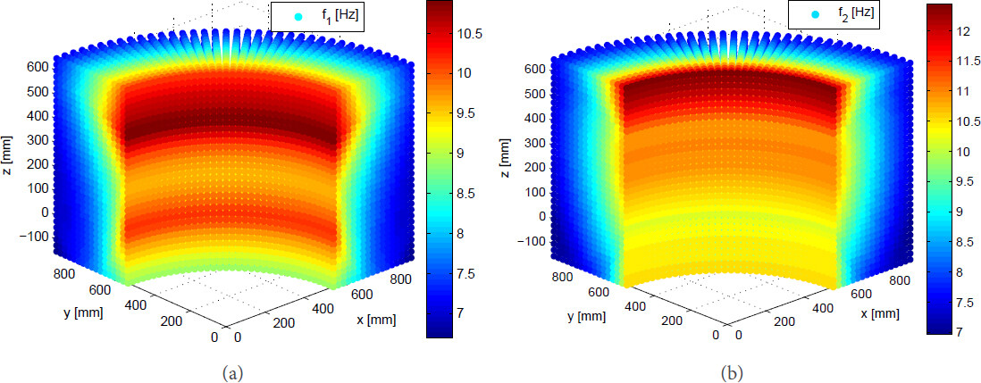
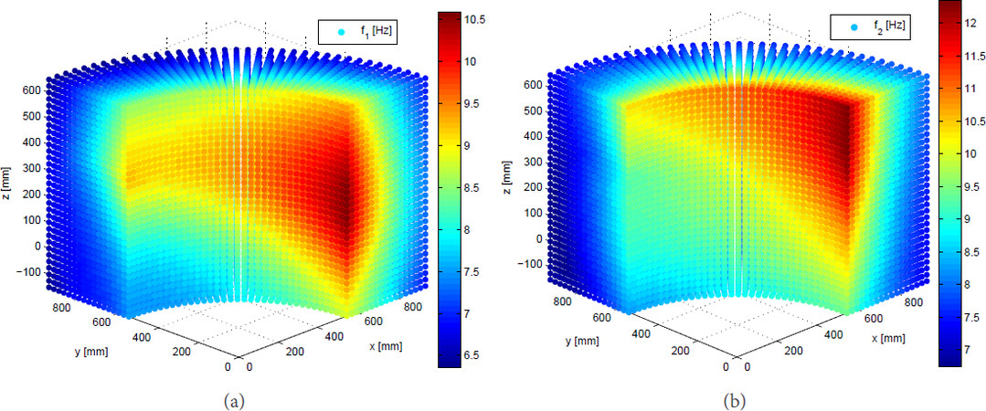
Figure 5. The natural frequency with constant-orientation [0, π/20]: (a) first order; and (b) second order.
Let the end-effector orientation follow the ZXZ Euler convention; the distributions of the first- and second-order natural frequencies over workspace are displayed in Figures 4 and 5 when the end-effector remains vertical and horizontal, respectively. It can be observed that the nonsymmetric distributions of the natural frequencies in Figure 5 are different from the symmetric ones in Figure 4. This is because the robot configurations are not axisymmetric about the vertical direction with the vertical end-effector, leading to different inverse kinematic solutions of such a 5-dof robotic arm, which are different from the axisymmetric robot configurations with horizontal end-effector. As the mass and stiffness matrices of the robot are configuration dependent, non-symmetric distributions of natural frequencies in Figure 5 occur. These two figures show that the first two orders of natural frequencies increase with the increasing z coordinates but with decreased x and y coordinates, namely both the first and second frequencies increases from the workspace boundaries to the origin of the global coordinate systems. As displayed in Figure 4, when the end-effector remains vertical, the natural frequencies have the same varying trend in any vertical cross-section of the workspace. By contrast, the first- and second-order frequencies become smaller counterclockwise within the workspace when the end-effector is in the horizontal configuration, as shown in Figure 5. Moreover, it is found that the differences among the frequencies of the manipulator in different configurations are not so large, which means that the robotic arm has close frequencies inside the overall workspace.
4.2. Sensitivity analysis
Sensitivity analysis can be used to evaluate the influence of the geometric parameters and design variables to the manipulator performances. Based on the elastodynamic equation, there exists
Upon differentiation of Equation (49), the derivative equation with respect to a variable δ is obtained as follows:
Taking the dot-product on both sides of Equation (50) yields
From
we have
or
Figure 6 illustrates the sensitivity of the first-order natural frequency to the first two active joints with constant orientation [0, π/2, 0]. It is found that the first-order natural frequency is much more sensitive to the second joint, particularly in the upper and lower workspace regions, which implies that the robots dynamic performance can be improved by replacing the second joint with a stiffer actuator. It is noted that the distributions of sensitivity coefficients are not symmetric, which is because the robot configurations are not axisymmetric about the vertical direction when the robot end-effector moves with some constant orientations, since the robot under study is a 5-dof robotic arm. Moreover, if a payload with more mass were exerted to the robot, it could be predicted that the sensitivity coefficients will be increased with very tiny varying trends, compared to the present results.
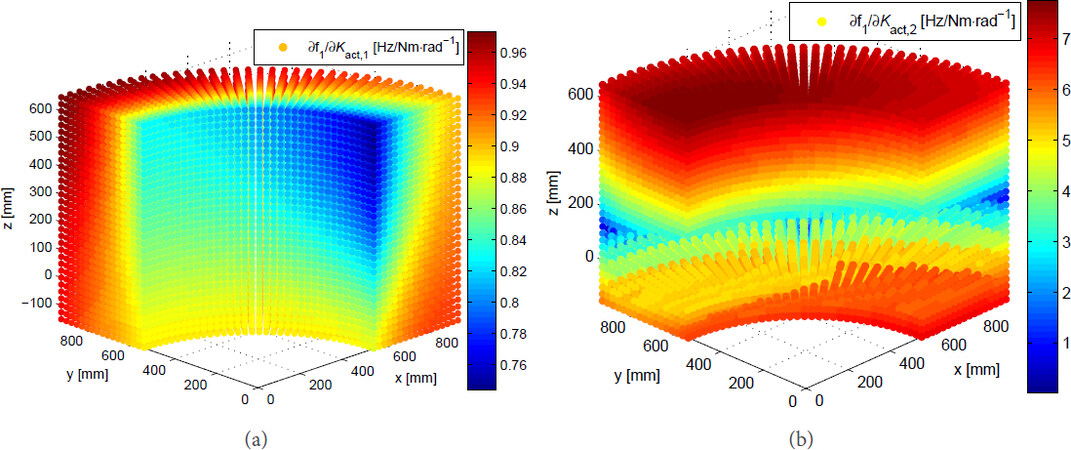
Figure 6. Sensitivities of the first-order natural frequency to the joint stiffness: (a) Joint 1; and (b) Joint 2.
4.3. Dynamic analysis of loaded system
With the payload 5 kg applied to the end-effector of the robotic arm, they constitute a new dynamic system and the solved frequencies with constant-orientation [0, π/2, 0] are illustrated in Figure 7, from which it is observed that the frequencies of the loaded robotic system decrease about 20% compared to Figure 5. Table 4 lists the average frequencies[46] within the constant-orientation workspace defined by
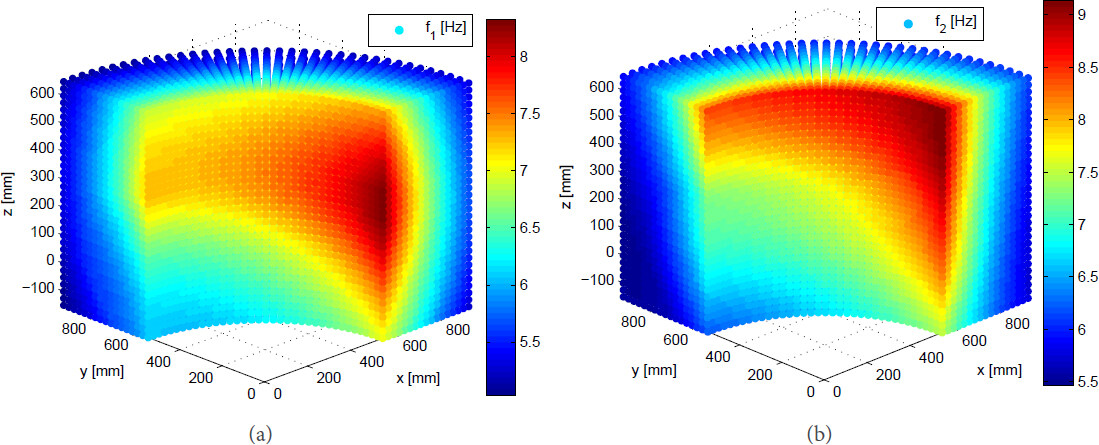
Figure 7. The frequencies with payload at constant-orientation [0, π/2, 0]: (a) first order; and (b) second order.
The mean frequency (Hz) within the dexterous workspace
| Natural frequency | 7.9404 | 8.9579 | 19.0263 | 84.9292 | 136.1418 | 300.6579 |
| Frequency with payload | 5.9538 | 6.5358 | 15.2772 | 55.8998 | 86.6291 | 276.5956 |
where Ω stands for the workspace volume. Different from the traditional industrial robots with low frequencies, the high order frequencies have large values to make the manipulator achieve high-speed motion. Compared to the average natural frequencies, the frequencies of the robotics with payload reduce 10%–40% for the six orders of frequencies. From the view of kineto-elastodynamic characteristics, the difference between the frequency of the loaded system and its natural frequency could be a consideration in the design of the mechanical system, where the smaller difference implies higher rigidity and higher payload capability.
Assuming that the motion of the robotic arm follows the trajectory (unit: mm) defined by
where the end-effector keeps constant-orientation [0, π, 0] and the motion period T = 0.5s is divided into 1024 intervals, Figure 8 shows the displacement responses of the end-effector, from which it is seen that the linear elastic displacement responses are close, whenever the robotic arm is under loaded and unloaded working modes. The angular displacements of the end-effector generate relatively large differences. The largest deformations appear around 0.3 s where the end-effector is located in the middle layer of the workspace, approximately z = 250 mm.
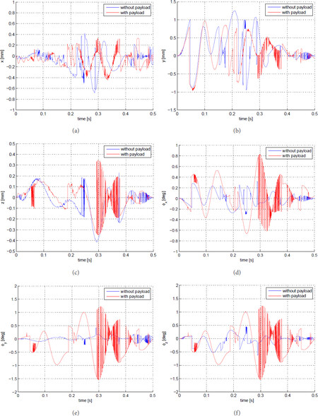
Figure 8. Displacement responses of the end-effector: (a) x direction; (b) y direction; (c) z direction; (d) ϕx direction; (e) ϕy direction; and (f) ϕz direction.
Figure 9 shows the comparison of the joint angular displacements between the numerical simulation and experimental measurements along previous trajectory, where the experimental data are read from the motor encoders. Due to the frictions and time-varying disturbance in the joints, the experimental curve profiles have more fluctuations and larger vibration amplitudes than the simulation ones. On the other hand, the comparison shows that the differences between these two curves are small, thus, the built analytical model can be acceptable for dynamic analysis of the robots.
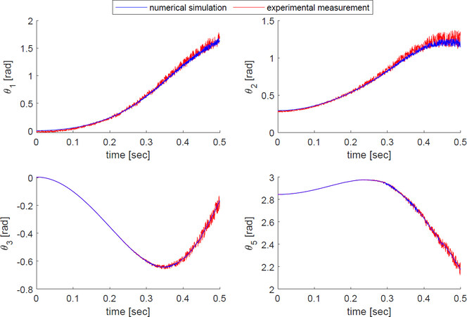
Figure 9. Comparison of the joint angular displacements under loaded mode.
5. Conclusion
This paper presents the elastodynamic characteristics of a 5-dof lightweight robotic arm. The main contribution is that a systematic approach of elastodynamic analysis for serial robotic manipulators is formulated, where the arm gravity and external load are taken into account to investigate the dynamic behaviors of the robotic arms, i.e., frequencies, sensitivity analysis, and displacement responses, with auxiliary payloads exerted to the robot. The modeling in this work eases the evaluation of elastodynamics of the manipulator at a large number of postures as the elastodynamic aspect is usually time-consuming. As the mass and stiffness matrices are posture dependent, the proposed method can effectively provide a symbolic calculation and achieve the modal analysis along an operating trajectory. Moreover, such a model can compute the additional mass or evaluate the influence of an isolator to the system more precisely to eliminate/reduce vibration in the vibration control. The developed model can be used in either performance evaluation or design optimization.
The frequencies of the loaded robotics are visualized within the representative workspace regions to show the overall dynamic performance and compare them with the natural frequencies. The comparison reveals that the studied robot keeps relatively high rigidity with high payload ratio. It is found from sensitivity analysis that the natural frequency can effectively increase by improving the second joint stiffness. Based on the displacement responses analysis, the payload has a slight influence on the translational elastic displacements of this robotic system, although it leads to reduced frequencies, while the effect on the rotation deflections cannot be ignored. In the future, the developed model will be integrated into its control system and an optimum redesign of the robotics will be conducted.
Declarations
Authors' contributions
The author contributed solely to the article.
Availability of data and materials
Not applicable.
Financial support and sponsorship
This work was supported by Natural Science Foundation of Liaoning Province (Grant No. 20180520028).
Conflicts of interest
The author declared that there are no conflicts of interest.
Ethical approval and consent to participate
Not applicable.
Consent for publication
Not applicable.
Copyright
© The Author(s) 2021.
Supplementary Materials
REFERENCES
1. Ivlev O, Martens C, Graeser A. Rehabilitation Robots FRIEND-I and FRIEND-II with the dexterous lightweight manipulator. Technology and Disabilily 2005;17:111-23.
2. Bien Z, Chung MJ, Chang PH, Kwon DS. Integration of a Rehabilitation Robotic System (KARES II) with Human-Friendly Man-Machine Interaction Units. Auton Robot 2004;16:165-91.
3. Mahoney RM. The Raptor wheelchair robot system. In: Mokhtari M, editor. Integration of Assistive Technology in the Information Age. IOS press; 2001. pp. 135-41.
4. Universal Robots. Available from https://www.universal-robots.com/GB/Cases.aspx.
5. Wu G, Shen H. In: Introduction. Singapore: Springer Singapore; 2021. pp. 1-15.
6. Hoevenaars AG, Krut S, Herder JL. Jacobian-based natural frequency analysis of parallel manipulators. Mech Mach Theory 2020;148:103775.
7. Briot S, Pashkevich A, Chablat D. On the optimal design of parallel robots taking into account their deformation and natural frequencies. In: ASME IDETC & CIE Conf. vol. DETC2009-86230. San Diego, California, USA: 2009. pp. 367-76.
8. Siciliano B, Khatib O. Springer Handbook of Robotics. Springer; 2016.
9. Cammarata A, Condorelli D, Sinatra R. An algorithm to study the elastodynamics of parallel kinematic machines with lower kinematic pairs. ASME J Mech Robot 2013;5:011004.
10. Dwivedy SK, Eberhard P. Dynamic analysis of flexible manipulators, a literature review. Mech Mach Theory 2006;41:749-77.
11. Briot S, Khalil W. In: Ceccarelli M, editor. Dynamics of Parallel Robots, vol. 35 of Mechanisms and Machine Science. Springer International Publishing AG Switzerland; 2015.
12. Khalil W, Gautier M. Modeling of mechanical systems with lumped elasticity. In: Proceedings 2000 ICRA. Millennium Conference. IEEE International Conference on Robotics and Automation. Symposia Proceedings (Cat. No. 00CH37065). vol. 4. San Francisco, CA, USA: IEEE; 2000. pp. 3964-69.
13. Wittbrodt E, Adamiec-Wójcik I, Wojciech S. Dynamics of Flexible Multibody Systems: Rigid Finite Element Method. Foundations of Engineering Mechanics. Springer Science & Business Media; 2007.
14. Briot S, Khalil W. Recursive and symbolic calculation of the elastodynamic model of flexible parallel robots. Int J Robot Res 2014;33:469-83.
15. Taghvaeipour A, Angeles J, Lessard L. Elastodynamics of a two-limb Schönflies motion generator. Proc Ins Mech Eng Part C J Mech Eng Sci 2015;229:751-64.
16. Boyer F, Coiffet P. Symbolic modeling of a flexible manipulator via assembling of its generalized Newton-Euler model. Mech Mach Theory 1996;31:45-56.
17. Rognant M, Courteille E, Maurine P. A systematic procedure for the elastodynamic modeling and identification of robot manipulators. IEEE Trans Robot 2010;26:1085-93.
18. Bauchau OA. Flexible Multibody Dynamics, vol. 176 of Solid Mechanics and Its Applications. Springer Science & Business Media; 2010.
19. de Jalon JG, Bayo E. Kinematic and Dynamic Simulation of Multibody Systems: the Real-time Challenge. Springer Science & Business Media; 2012.
20. Wu G, Shen H. In: Ding H, Sun R, editors. Parallel PnP Robots, vol. 7 of Research on Intelligent Manufacturing. Springer, Singapore; 2021.
21. Ku DM, Chen LW. Kineto-elastodynamic vibration analysis of robot manipulators by the finite element method. Comput Struct 1990;37:309-17.
22. Salisbury JK. Active stiffness control of a manipulator in cartesian coordinates. In: 1980 19th IEEE Conference on Decision and Control including the Symposium on Adaptive Processes. Albuquerque, NM, USA: 1980. pp. 95-100.
24. Wittbrodt E, Adamiec-Wójcik I, Wojciech S. Dynamics of Flexible Multibody Systems. Springer; 2006.
25. Quennouelle C, Gosselin C. Kinematostatic modeling of compliant parallel mechanisms. Meccanica 2011;46:155-69.
26. El-Khasawneh BS, Ferreira PM. Computation of stiffness and stiffness bounds for parallel link manipulators. Int J Mach Tool Manuf 1999;39:321-42.
27. Gosselin CM, Zhang D. Stiffness analysis of parallel mechanisms using a lumped model. Int J Robot Autom 2002;17:17-27.
28. Dai J, Ding X. Compliance analysis of a three-legged rigidly-connected platform device. ASME J Mech Des 2006;128:755-64.
29. Majou F, Gosselin C, Wenger P, Chablat D. Parametric stiffness analysis of the Orthoglide. Mech Mach Theory 2007;42:296-311.
30. Pashkevich A, Chablat D, Wenger P. Stiffness analysis of overconstrained parallel manipulators. Mech Mach Theory 2009;44:966-82.
31. Kövecses J, Angeles J. The stiffness matrix in elastically articulated rigid-body systems. Multi Syst Dyn 2007;18:169-84.
32. Quennouelle C, Gosselin CM. Stiffness Matrix of Compliant Parallel Mechanisms. In: Lenarčič J, Wenger P, editors. Advances in Robot Kinematics: Analysis and Design. Springer Netherlands; 2008. pp. 331-41.
33. Tyapin I, Hovland G. Kinematic and elastostatic design optimisation of the 3-DOF Gantry-Tau parallel kinematic manipulator. Modeling, Identification and Control 2009;30:39-56. DOI
34. Cammarata A, Caliò I, D'Urso D, et al. Dynamic stiffness model of spherical parallel robots. J Sound Vib 2016;384:312-24.
35. Wu L, Wang G, Liu H, Huang T. An approach for elastodynamic modeling of hybrid robots based on substructure synthesis technique. Mech Mach Theory 2018;123:124-36.
36. Wu J, Li T, Wang J, Wang L. Stiffness and natural frequency of a 3-DOF parallel manipulator with consideration of additional leg candidates. Robot Auton Syst 2013;61:868-75.
37. Lara-Molina FA, Koroishi EH, Costa TL. Elastodynamic Performance of a Planar Parallel Mechanism Under Uncertainties. In: International Symposiu on Multibody Systems and Mechatronics. Springer; 2017. pp. 183-92.
38. Wu G, Zhao W, Zhang X. Optimum time-energy-jerk trajectory planning for serial robotic manipulators by reparameterized quintic NURBS curves. Proc Ins Mech Eng Part C J Mech Eng Sci 2021;235:4382-93. DOI
39. Denavit J, Hartenberg RS. A kinematic notation for lower-pair mechanisms based on matrices. ASME J Appl Mech 1955;22:215-21.
40. Tsai LW. Robot Analysis: The Mechanics of Serial and Parallel Manipulators. John Wiley & Sons; 1999.
41. Ranjbaran F, Angeles J, González-Palacios MA, Patel RV. The mechanical design of a seven-axes manipulator with kinematic isotropy. J Intell Robot Syst 1995;14:21-41.
42. Pashkevich A, Klimchik A, Chablat D. Enhanced stiffness modeling of manipulators with passive joints. Mech Mach Theory 2011;46:662-79.
43. Wu G, Bai S, Kepler J. Mobile platform center shift in spherical parallel manipulators with flexible limbs. Mech Mach Theory 2014;75:12-26.
44. Rao SS. Mechanical Vibrations. 4th ed. Prentice Hall; 2003.
45. Dong C, Liu H, Huang T, Chetwynd DG. A screw theory-based semi-analytical approach for elastodynamics of the Tricept robot. ASME J Mech Robot 2019;11:031005.
Cite This Article
Export citation file: BibTeX | RIS
OAE Style
Wu G. On the elastodynamics of a five-axis lightweight anthropomorphic robotic arm. Intell Robot 2021;1(2):99-115. http://dx.doi.org/10.20517/ir.2021.11
AMA Style
Wu G. On the elastodynamics of a five-axis lightweight anthropomorphic robotic arm. Intelligence & Robotics. 2021; 1(2): 99-115. http://dx.doi.org/10.20517/ir.2021.11
Chicago/Turabian Style
Wu, Guanglei. 2021. "On the elastodynamics of a five-axis lightweight anthropomorphic robotic arm" Intelligence & Robotics. 1, no.2: 99-115. http://dx.doi.org/10.20517/ir.2021.11
ACS Style
Wu, G. On the elastodynamics of a five-axis lightweight anthropomorphic robotic arm. Intell. Robot. 2021, 1, 99-115. http://dx.doi.org/10.20517/ir.2021.11
About This Article
Special Issue
Copyright

Data & Comments
Data


 Cite This Article 21 clicks

 Like This Article 31
likes
Like This Article 31
likes


Comments
Comments must be written in English. Spam, offensive content, impersonation, and private information will not be permitted. If any comment is reported and identified as inappropriate content by OAE staff, the comment will be removed without notice. If you have any queries or need any help, please contact us at support@oaepublish.com.