Autonomous navigation in unknown environment using sliding mode SLAM and genetic algorithm

1. Introduction

2. Sliding mode slam

SLAM gives the robot position and environment map at the same time. At time k, the state is $$\mathbf{x}_{k}^{r}=\left(x_{k}, y_{k}, \theta_{k}\right)$$ where (x_k, y_k) is the position and θ_k is the orientation of the robot. $$\mathbf{x}_{k}^{m}=\left(\mathbf{m}_{k}^{1}, \mathbf{m}_{k}^{2}, \ldots, \mathbf{m}_{k}^{{L}}\right)^{T}$$ are landmarks, with $$ \mathbf{m}_{k}^{i}=\left(x_{k}^{i}, y_{k}^{i}\right)^{T} $$ the ith landmark. We assume the true location is time-invariant.

X_k has two parts: the robot $$\mathbf{x}_{k}^{r}$$ and the landmarks $$\mathbf{x}_{k}^{m}$$ The state equation is

where f () is the robot dynamics, W_k is the noise, and u_k is the robot control. Since $$\mathbf{x}_{k}^{m}$$ is not influenced by motion noise, the noise is [W_k, 0]^T.

Z_k is defined as the position between the robot and the landmark, whose model is

where h() is the geometry and vⁱ_k is the noise. Here, w_k and vⁱ_k are not Gaussian noises. We assume w_k and vⁱ_k are bounded.

To estimate x_k in Equations (1) and (2), EKF is needed. We linearize the state model in Equation (1) and the observation model in Equation (2) as

where $$\nabla \mathbf{F}_{k}=\left.\frac{\partial \mathbf{F}}{\partial \mathbf{x}_{k}}\right|_{\mathbf{x}_{k}=\hat{\mathbf{x}}_{k}}, \nabla \mathbf{h}_{k}=\left.\frac{\partial \mathbf{h}}{\partial \mathbf{x}_{k}}\right|_{\mathbf{x}_{k}=\hat{\mathbf{x}}_{k}}, O_{1}\left[\left(\mathbf{x}_{k}-\hat{\mathbf{x}}_{k}\right)^{2}\right], \hat{\mathbf{x}}_{k}$$ is the estimation of x_k.

Prediction. The estimation $$\hat{\mathbf{x}}_{k+1}$$ is based on past states, control, and landmarks:

where R₁ is the covariance of W_k, R₁ = E {[W_k – E (W_k)] [W_k – E (W_k)]^T}.

Correction. The new state is based on predicted states, landmarks, and current observations:

The motivations of using sliding mode modification to the EKF bases SLAM based are the following:

(1) The noises w_k and $$\mathbf{V}_{k}^{i} $$ in Equations (1) and (2) are not Gaussian.

(2) There are linearization error terms, $$ O_{1}\left[\left(\mathbf{x}_{k}-\hat{\mathbf{x}}_{k}\right)^{2}\right] \text { and } O_{2}\left[\left(\mathbf{x}_{k}-\hat{\mathbf{x}}_{k}\right)^{2}\right] $$, in Equation (3), and the traditional EKF-based methods do not work well for these errors.

We use the sliding mode method to estimate the robot state $$\mathbf{X}_{k}^{r} $$ and the landmark $$\mathbf{X}_{k}^{m} $$

Sliding modes have a number of attractive features, and thus have long been in use for solving various control problems. The basic idea behind design of system with sliding mode is the following two steps: (1) a sliding motion in a certain sense is obtained by an appropriate choice of discontinuity surfaces; and (2) a control is chosen so that the sliding modes on the intersection of those discontinuity surface would be stable. A general class of discontinuous control u (x, t) is defined by the following relationships:

where the functions u⁺ (x, t) and u^– (x, t) are continuous.

The function S (x) is the discontinuity surface (subspace). The objective of the sliding mode control is to design some switching strategy of the continuous control u⁺ (x, t) and u^– (x, t), such that

In this paper, the sliding surface is defined by the SLAM estimation error as

Here, the discontinuity surface is e (k) = [e₁… e_n]. We consider the following positive definite function,

where P is diagonal positive definite matrix, P = P^T > 0. The derivative of V is

The motion e (k) satisfies

where $$sgn[e (k)]=\left[sgn\left(e_{1}\right), \ldots, sgn\left(e_{n}\right)\right]^{T}, sgn\left(e_{i}\right)=\left\{\begin{array}{l} 1 \text { with } e_{i}(x)>0 \\ -1 \text { with } e_{i}(x)<0 \end{array}\right.$$, sgn (0) = 0, then (10) is

because P = diag {p_i}, p_i > 0, and e_i × sgn (e_i) = |e_i|

Thus, $$\dot{V}\le 0$$ By Barbalat’s lemma^[48], the estimation error is e (k) → 0.

The classical SLAM in Equations (4) and (5) is modified by the sliding surface in Equation (11). The sliding mode control can be regarded as a compensator for Equation (4):

where ρ is a positive constant. The correction step is the same as EKF in Equation (5). The sliding mode SLAM is shown in Figure 1. Here, the estimation error, e (k), is applied to the sliding surface to enhance the robustness in the prediction step with respect to the noise and disturbances.

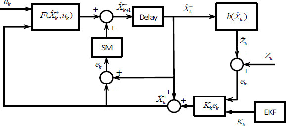
Figure 1. Sliding mode simultaneous localization and mapping.

It is the discrete-time version of Equation (6). We give the stability analysis of this discrete-time sliding mode SLAM at the end of this section.

For the mobile robot, the sliding mode SLAM can be specified as follows. We define a critical distance d_min to limit the maximal landmark density. It can reduce false positives in data association and avoid overload with useless landmarks. If the new landmark is far from the other landmarks on the map, then the landmark is added; otherwise, it is ignored. If the distance between the new landmark X_k+1 = [x_m+1,y_m+1] and the others is bigger than d_min, it should be added into x_k, i.e.,

It can be transformed into an absolute framework as

The nonlinear transformation function T also applies to the uncertainties. We approximate the transformation T by the linearization. P_k can be expressed as

where

with $$\begin{array}{l} \nabla \mathbf{T}=\left(\begin{array}{ccc} \mathbf{I}_{r} & \mathbf{0} & \mathbf{0} \\ \mathbf{0} & \mathbf{I}_{m} & \mathbf{0} \\ \nabla \mathbf{g}_{x} & \mathbf{0} & \nabla \mathbf{g}_{z} \end{array}\right), \nabla \mathbf{g}_{x}:=\frac{\partial \mathbf{g}}{\partial \mathbf{x}_{k}^{r}}\left(\mathbf{X}_{k}, \mathbf{z}_{k}\right), \nabla \mathbf{g}_{z}:=\frac{\partial \mathbf{g}}{\partial \mathbf{Z}}\left(\mathbf{X}_{k}, \mathbf{z}_{k}\right). \\ \end{array}$$

For the motion part, we use the Ackerman vehicle model ^[49]

where W_k is the process noise, v_k is the linear velocity, α_k is the steering angle, T_k is the sample time, and b_a is the distance between the front and the rear wheels.

At the beginning of map building, the vector $$ \hat{\mathbf{X}}_k $$ only contains the robot states without landmarks. As exploration increases, the robot detects landmarks and decides if it should add these new landmarks to the state.

where x, y, z, and m are defined in Equations (1) and (2),

We exploit the same property in the sliding SLAM. The landmarks with fewer corrections are removed from the state vector.

where $$G_{x}=\left(\begin{array}{cccc} 1 & 0 & 0 & 0 \cdots 0 \\ 0 & 1 & 0 & 0 \cdots 0 \\ 0 & 0 & 1 & \underbrace{0 \cdots 0}_{2 N} \end{array}\right), \sigma_{k} $$ is the compensator, and

This sliding SLAM algorithm is given in the following algorithm.

The discrete-time sliding mode SLAM in Equation (19) can be written as

where $$ \hat{F}=G_{x}^{T}\left[\begin{array}{c} u_{k, v} \delta_{t} \cos \left(\mathbf{X}_{k, \phi}^{r}\right) \\ u_{k, v} \delta_{t} \sin \left(\mathbf{X}_{k, \phi}^{r}\right) \\ u_{k, \gamma} \delta_{t} \end{array}\right], e(k)=\mathbf{X}_{k}-\hat{\mathbf{X}}_{k}, \sigma_{k}=\rho \times sgn[e(k)]$$

The correction step for $$\hat{\mathbf{x}}_{k+2}$$ is the same as EKF:

where $$ C_{k}=\nabla \mathbf{h}_{k}=\left.\frac{\partial \mathbf{h}}{\partial \mathbf{x}_{k}}\right|_{\mathbf{X}_{k}=\hat{\mathbf{x}}_{k}} $$

The error dynamic of this discrete-time sliding mode observer is

where $$d_{k}=\hat{F}\left(\hat{\mathbf{X}}_{k}, \mathbf{u}_{k}\right)+\xi_{k}$$ is bounded uncertainty, $$\left\|d_{k}\right\|^{2} \leq \bar{d}, A_{k}=\nabla \mathbf{F}_{k}=\left.\frac{\partial \mathbf{F}}{\partial \mathbf{x}_{k}}\right|_{\mathbf{x}_{k}=\hat{\mathbf{x}}_{k}}$$, and K_k is the gain of EKF in Equation (21).

The next theorem gives the stability of the discrete-time sliding mode SLAM.

Theorem 1If the gain of the sliding mode SLAM is positive, then the estimation error is stable, and the estimation error converges to

where $$||\sigma_{k}||^{2} \leq \bar{\rho}, \sigma_{k}\left\|d_{k}\right\|^{2} \leq \bar{s}, \mathbf{P}_{k+2}$$ is the gain of EKF in Equation (21), $$0 <\alpha=\frac{1}{\left(1+\bar{p} \bar{a}^{2} / \underline{q}\right)(1+\bar{k} \bar{c}+\lambda)}< 1, \quad \underline{p}I \le \mathbf{P}_{k+2} \le \bar{p}I,~and~\underline{q}I \le {R_1}.$$

Proof 1Consider the Lyapunov function as

where P_k+2 is the prior covariance matrix in Equation (21), and P_k+2> 0. From Equation (22),

Because $$ ||\sigma_{k}||^{2} \leq \bar{\rho},\left\|d_{k}\right\|^{2} \leq \bar{s}$$, the last term on the right side of Equation (25) is

where $$\lambda_{\max }\left[\mathbf{P}_{k+1}^{-1}\right]$$ is the maximum eigenvalue of $$\mathbf{P}_{k+1}^{-1}$$

The second term of Equation (25) is

where K_k is the gain of EKF in Equation (5). In view of the matrix inequality

which is valid for any X, Y ∊ $$ \Re^{n \times k} $$and for any positive definite matrix 0 < Λ = Λ^T ∊ $$ \Re^{n \times n} $$, the first term of Equation (27) is

We apply the sliding mode compensation in Equation (20) to the second term of Equation (27):

where l_ij are the elements of the matrix$$\Upsilon,~\Upsilon_{k}=\mathbf{P}_{k+1}^{-1}\left[A_{k}\left(I-\mathbf{K}_{k} C_{k}\right)\right] . $$When the the orientation θ_k is not big sin θ_k ≈ 0, cos θ_k ≈ 0,

Thus, the second term of Equation (27) is negative.

The first term on the right side of Equation (25) has the following properties:

(I - K_kC_k) is invertible, and we have

According to EKF,

Thus,

By the following matrix inversion lemma,

where Γ and Ω are two non-singular, matrices,

Using Equation (32) and defining L = (1 –K_kC_k),

Now,

Hence,

Combining the last term of Equation (29) with the first term on the right side of Equation (25),

where $$ \left\|A_{k}\right\|=\sqrt{tr\left(A_{k} A_{k}\right)} \leq \bar{a},\left\|C_{k}\right\|=\sqrt{tr\left(C_{k} C_{k}\right)} \leq \bar{c},\left\|\mathbf{K}_{k}\right\|=\sqrt{tr\left(\mathbf{K}_{k} \mathbf{K}_{k}\right)} \leq \bar{k}, \lambda=\left\|\Lambda^{-1}\right\|, \underline{p} I \leq \mathbf{P}_{k+2} \leq \bar{p} I, \underline{q} I \leq R_{1} $$, and

Combining Equation (26), the first term of Equation (29), and Equation (34),

Thus,

where$$\kappa =\lambda_{\mathrm{max}}[{\mathbf{P}}_{k+1}^{-1}](\bar{\rho}+\bar{s})+\lambda_{\mathrm{max}}[\Lambda]\bar{\rho} $$. If

then V_k+1– V_k ≤ 0, ||e (k)|| decreases. Thus, ||e (k)|| converges to Equation (23).

3. Genetic algorithm and slam for path planning

Path planning is one key problem of autonomous robots. Here, the map is built by the sliding mode SLAM:

• The obstacle set is defined by B_obs(t).

• The position is x_r(t), B_free(t) = B\B_obs(t).

• The path planning is f (x (t), xs, x_T),x_s = x_r(t).

The previous map is B_free(t), which requires the path f(x(t),xs,x_T).

We assume the previous map is obstacle-free, the initial point is x_s, the target point is x_T ∊ B,

the obstacle is $$ B_{obs}=\frac{B}{B_{free}}, z_{r}$$ is the shape of the robot, and A(z_r) is the area of the robot. The objective of the path planning is to find a path f(x,x_s,x_T) ∊ B_free that allows the robot to navigate.

D is defined as the search space. We use the GA to find an optimal trajectory f (x, x_s, x_T), such that

Here, we use stochastic search for GA, and each iteration includes: reproduction or selection, crossing or combination, and mutation. The population is $$ P(k)=\left\{S_{1}^{k}, S_{2}^{k}, \ldots, S_{m}^{k}\right\} $$ with m being the size of the population that represents the possible solutions:

(1) Every chromosome $$ S_{i}^{t} $$ has a solution in D.

(2) Crossing the chromosomes. An intersection in $$ S_{a}^{k}=\left[\varsigma_{l}^{a}, \varsigma_{l-1}^{a}, \ldots, \varsigma_{2}^{a}, \varsigma_{1}^{a}\right] \text { and } S_{b}^{k}=\left[\varsigma_{l}^{b}, \varsigma_{l-1}^{b}, \ldots, \varsigma_{2}^{b}, \varsigma_{1}^{b}\right] $$ belongs to D, such that $${S}_{a}^{t} \cap S_{b}^{t} \neq {0}$$; then,

where $$ S_{a^{\prime}}^{t}$$ and $$ S_{b^{\prime}}^{t}$$ are the next generation from two compatible chromosomes by crossing.

(3) Mutation. It replace a number of chromosomes by chromosomes in D.

The mutation operation is calculated by the fitness of each chromosome, $$ P(M u t)=\left[fit\left(S_{1}^{M u t}\right), fit\left(S_{2}^{M u t}\right), \ldots, fit\left(S_{n}^{M u t}\right)\right] $$ where n is the number of mutations and fit uses the

Euclidean distance. The total fitness is $$ Fit =\displaystyle \sum_{i=1}^{n} f i t\left(S_{i}^{M u t}\right) $$ Therefore, the probability of selection p_i, of a chromosome S_i for i = 1, 2,…, n is

An optimal solution p^M in D is mutated by

In the mutation operation, an optimal solution with p^M = 1 is a global solution if n → ∞. To prove the convergence, we use a Markov chain, as shown in Figure 2. Each chromosome can move from Q_ij to the state Q_i(j+1). The moving probability is ρ_ji,ik > 0, i = 1, 2, …,n, k,j = 1, 2, …,m.

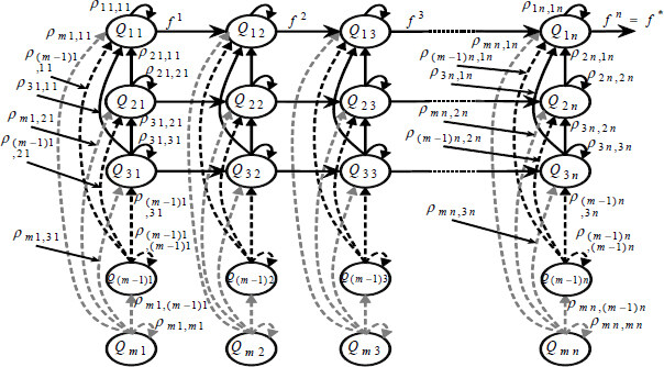
Figure 2. Roadmap genetic algorithm model as a finite Markov chain.

The operators, selection, crossing, and mutation create P(k) with p^k. It preserves the best chromosomes of P(k – 1). P(k + 1) in the population P(k) can be regarded as the Markov transition:

Theorem 2If GA for the roadmap is an elitist process, then the probability of p*in D is exponential.

Proof 2The iteration Q₁ is changed with the chromosomes when genetic process is elitist,

where n is the size of the population. If for all α, β ∊ D, there is 0 < τ ≤ msuch that H^τ (α, β) ≥ ∊ > 0, then

This implies that, given certain state Q_t, the probability of transition in time t between t and t + m is at least ∊,

Without loss of generality, the transition in the iteration k + 1 is

Using Equation (42), we have

where $$ H\left(P_{t} \neq p^{*} \forall 0< t \leq 0\right)=1, $$ then

Since 0 < ∊ ≤ 1, the algorithm converges exponentially to p* in: population size n and iteration number k.

The algorithm of the SLAM-based roadmap GA for the path planning is as follows.

4. Autonomous navigation

Our AN uses both sliding mode SLAM (Algorithm 1) and the roadmap GA method (Algorithm 2). The autonomous navigation algorithm is:

The PP needs the map, robot position, and target. This information is given by the sliding mode SLAM algorithm. When the algorithm falls into a local solution, we use the ComputeOutsideLocal function to provide another S_n which is outside the local zone.

5. Comparisons

In this section, we use several examples to compare our method with the three other recent methods: the polar histogram method for path planning^[50], the grid method for path planning^[51], and SLAM with extended Kalman filter ^[52].

5.1. Simulations

The following simulations were implemented in partially unknown and completely unknown environments. The size of the environments was 100 m × 100 m, in which a solution was sought to find a trajectory from the initial point x_s to the target point x_T. The sliding mode gains were selected as ρ = diag ([0.1, …, 0.1]).

In the partially unknown environments, B_obs(0) ≠ θ. The path planning solution p* was partial because the environment B_obs(t) was variant in time. Figure 3 shows a partial solution p* from an initial point x_s to the objective point x_T for the partially unknown environment. Figure 4 shows the overall result of the robot navigation from point x_s to point x_T with the robust SLAM algorithm combined with the GA.

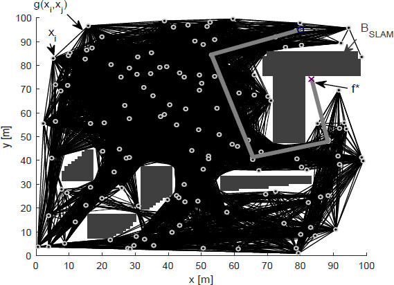
Figure 3. Sliding mode simultaneous localization and mapping.

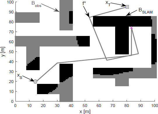
Figure 4. Autonomous navigation using sliding mode simultaneous localization and mapping and genetic algorithm method.

Here, the SLAM algorithm was used to construct the environment and find the position of the robot. At the beginning of navigation in the partially unknown environment, there was a planned trajectory of navigation through the GA algorithm; however, if an obstacle was found in the planned trajectory, the GA algorithm needed to be used to search for a new trajectory within the built environment by the SLAM, B_SLAM. The planned trajectory belonged to the set of obstacles that prevent reaching the goal, p* (B_obs(t); therefore, it was necessary to look for a new trajectory using RGA that allowed reaching the goal.

For the completely unknown environments, B_obs(0) = θ. In these environments, the SLAM algorithm was required to know the environment B_SLAM and the position of the robot; in this way, when an obstacle was found that contained the planned trajectory, a new trajectory with the GA algorithm was searched on the map

B_SLAM until the target point was reached the results obtained are shown in Figure 5. When we used the polar histogram method for path planning ^[50], only the local solutions could be found [Figure 6].

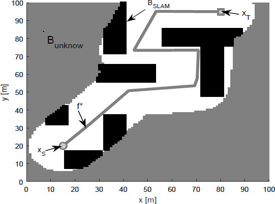
Figure 5. Sliding mode simultaneous localization and mapping and genetic algorithm in complete unknown environment.

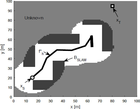
Figure 6. Polar histogram method in complete unknown environments.

Now, we compare the path lengths with the polar histogram method. The following density of the obstacles give the navigation complexity. The environment is free of obstacles when d_obs = 0. The whole environment is occupied by the obstacles when d_obs = 1. The index for the trajectory error is

(43) $$ \begin{equation} \begin{aligned} E_{PP}=\frac{effective~path - optimal~path}{100} \end{aligned} \end{equation} $$

We use the averages of the path length. The obstacles density is defined as

(44) $$ \begin{equation} \begin{aligned} d_{obs}=\frac{{\textstyle \sum_{n\in G_O}^{}S_{obs}(n)}}{||G_E||} \end{aligned} \end{equation} $$

The path length is defined as

(45) $$ \begin{equation} \begin{aligned} l_{sub}=\frac{effective~path}{optimal~path} \end{aligned} \end{equation} $$

The averages of the path lengths of our RA and the polar histogram are shown in Figure 7. When the density of obstacles was bigger, the path length of the polar histogram grew more quickly than that of ours. When the obstacle density d_obs was 0.3, E[l_sub, Navigation1] = 1.053, E[l_sub, Navigation2] = 1.152.

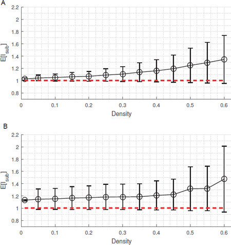
Figure 7. The average path length: (A) sliding mode simultaneous localization and mapping and genetic algorithm; and (B) polar histogram.

Next, we compare our method with the grid method^[51]. The comparison results are shown in Figure 8. For the task of navigating the robot or system in partially unknown or completely unknown environments, the SLAM algorithm was used to construct the environment and know the position of the robot. At the beginning of navigation in the partially unknown environment, there was a planned trajectory of navigation through the GA algorithm; however, if an obstacle were found in the planned trajectory, the GA algorithm needed to be used to search for a new trajectory within the built environment by the SLAM, B_SLAM.

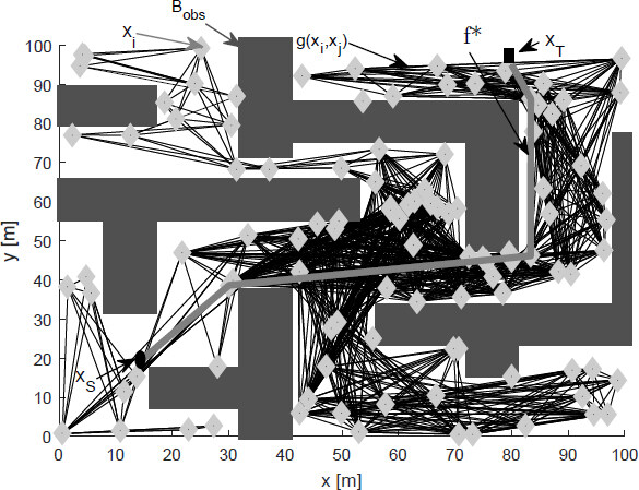
Figure 8. Sliding mode simultaneous localization and mapping (gray) and grid method (black)

The size of the environments was 100m× 100 m, in which a solution was sought to find a trajectory from the initial point x_s to the target point x_T.Figure 9 shows a path planning based on the proposed methods to find a solution f*. Here, 60 local targets were generated x_i with the search space D generated by the trajectories of the local targets that do not intersect with the set of obstacles; thus, it became an optimization problem to find an optimal path.

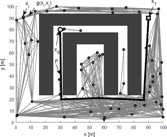
Figure 9. Sliding mode simultaneous localization and mapping based path planning (bold) and grid method (gray).

In an environment with previously generated obstacles of 100 m × 100 m, 120 possible targets were randomly generated x_i; therefore, the search space D would be all trajectories g(x_i,x_j) that do not intersect with the set of obstacles, where the roadmap genetic algorithm solved the problem of optimization to find a solution to the problem of path planning. For the problem presented above, we found that the proposed algorithm converged in 40 iterations. For these results, 100 tests were performed for each number of iterations and, as shown in Figure 10, the roadmap genetic algorithm converged with greater probability within 40 iterations.

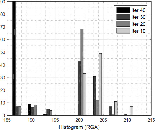
Figure 10. Performance of the genetic algorithm.

5.2. Application

The Koala mobile robot by K-team Corporation 2013 was used to validate our sliding mode SLAM. This mobile robot has encoders and one laser range finder. The position precision is less than 0.1 m.

The objective of this autonomous navigation is to force the robot to return to the starting point. The sliding mode SLAM was compared with SLAM with extended Kalman filter (EKF-SLAM) ^[52]

The initial covariance matrices are zero. The parameters of the algorithm are

$$ \begin{equation} \begin{aligned} \begin{array}{c} \rho=diag\left(\left[1 e^{-3}, 1 e^{-3}, 4 e^{-3}, 2 e^{-4}, \cdots, 2 e^{-4}\right]\right) \\ R_{1}=diag([0.05,0.05,0.005]), R_{2}=diag\left(\left[6 e^{-4}, 1 e^{-5}\right]\right) \end{array} \end{aligned} \end{equation} $$

Since the robot moves in the environment with bounded noise (see Figure 11), the noises are not Gaussian. Two different conditions are considered: (1) Koala robot pre-processes off-line the sensors data to reduce 90% noises; and (2) the computer uses sliding mode SLAM on-line.

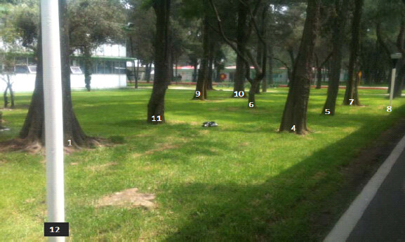
Figure 11. The environment of the autonomous navigation.

For the first case, Figure 12 shows that sliding mode SLAM and EKF-SLAM are similar. Both sliding mode SLAM and EKF-SLAM work well for the case with less noise. The robot can return to the starting point, and the map is constructed correctly.

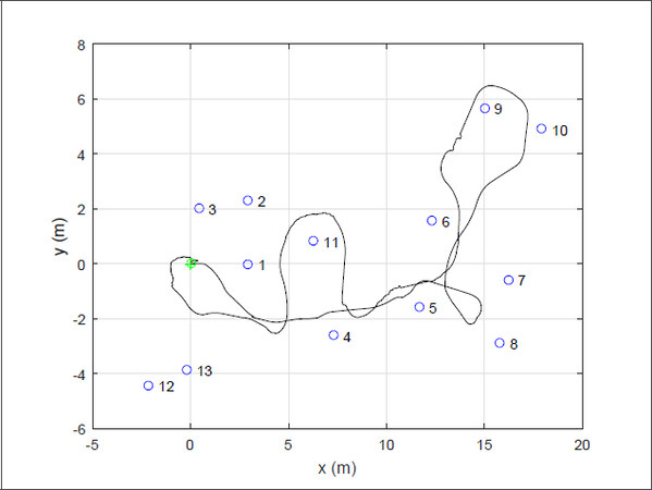
Figure 12. Results of extended Kalman filter simultaneous localization and mapping and sliding mode simultaneous localization and mapping with small noises.

For the second case, Figure 13 gives the results of EKF-SLAM. As can be seen, the robot cannot return to the starting point and the map is not exactly the same as the real one with EKF-SLAM because EKF-SLAM is sensitive to non-Gaussian noises.

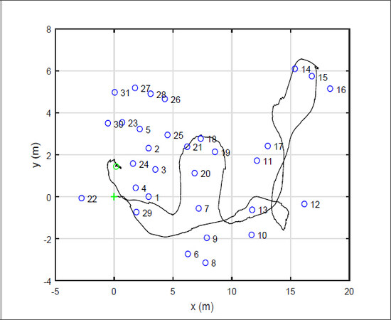
Figure 13. Results of extended Kalman filter simultaneous localization and mapping with noises.

Figure 14 shows the results with SM-SLAM. Under the same bounded noises, SM-SLAM works very well, because of the sliding mode technique.

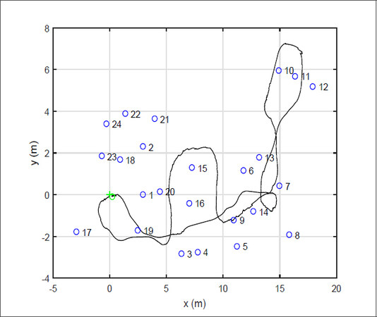
Figure 14. Results of sliding mode simultaneous localization and mapping with noise.

To compare the errors, we define the average of the Euclidean errors as

(46) $$ \begin{equation} \begin{aligned} E_{d}=\frac{1}{N_{T}} \displaystyle \sum_{k=1}^{N_{T}} \sqrt{\left(x_{k}-x_{k}^{*}\right)^{2}+\left(y_{k}-y_{k}^{*}\right)^{2}}, E_{a}=\frac{1}{N_{T}} \sum_{k=1}^{N_{T}}\left|\phi_{k}-\phi_{k}^{*}\right| \end{aligned} \end{equation} $$

where N_T is the data number; $$ x_{k}^{\ast}, y_{k}^{\ast}~\mathrm{and}~\phi_{k}^{\ast} $$ are real values for robot position and orientation; and x_k, y_k, and ϕ_k are estimations of them. Figure 15 shows the errors of EKF-SLAM and sliding mode SLAM. Obviously, the errors of EKF-SLAM increase quickly. Robots have better estimation in long distances with sliding mode SLAM.

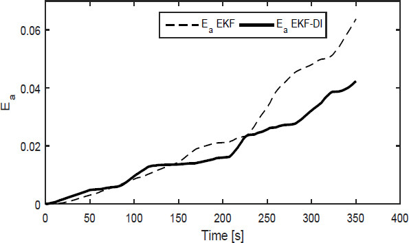
Figure 15. Direction estimation errors of sliding mode simultaneous localization and mapping (SLAM) and EKF-SLAM. EKF: Extended Kalman filter.

6. Conclusion

Navigation in unknown environments is a big challenge. In this paper, we propose sliding mode SLAM with genetic algorithm for path planning. Both sliding mode and GA can work in unknown environments. Convergence analysis is given. Two examples were applied to compare our model with other models, and the results show that our algorithm is much better in unknown environments.

REFERENCES

1. Luettel T, Himmelsbach M, Wuensche HJ. Autonomous ground vehicles—concepts and a path to the future. Proceedings of the IEEE 2012;100:1831-39.
2. Galceran E, Carreras M. A survey on coverage path planning for robotics. Rob Auton Syst 2013;61:1258-76.
3. Lowe DG. Distinctive image features from scale-invariant keypoints. Int J Comput Vis 2004;60:91-110.
4. Arel I, Rose DC, Karnowski TP. Deep machine learning-a new frontier in artificial intelligence research. IEEE Comput Intell Mag 2010;5:13-8.
5. Scheirer WJ, de Rezende Rocha A, Sapkota A, et al. Toward open set recognition. IEEE Trans Pattern Anal Mach Intell 2012;35:1757-72.
6. Ramos FT, Kumar S, Upcroft B, et al. A natural feature representation for unstructured environments. IEEE Trans Robot 2008;24:1329-40.
7. Lillywhite K, Lee DJ, Tippetts B, et al. A feature construction method for general object recognition. Pattern Recognition 2013;46:3300-14.
8. Chabini I, Lan S. Adaptation of the A* algorithm for the computation of fastest paths in deterministic discrete-time dynamic networks. IEEE trans Intell Transp Syst 2002;3:60-74.
10. Valencia R, Andrade-Cetto J. Mapping, planning and exploration with Pose SLAM. Berlin: Springer; 2018. pp. 60-84.
11. Wang X, Shi Y, Ding D, et al. Double global optimum genetic algorithm–particle swarm optimization-based welding robot path planning. Eng Optim 2016;48:299-316.
12. Jones M, Peet MM. A generalization of Bellman’s equation with application to path planning, obstacle avoidance and invariant set estimation. Automatica 2021;127:109510.
13. Rehman NU, Kumar K, Abro GeM. Implementation of an autonomous path plan-ning & obstacle avoidance UGV using SLAM. 2018 International Conference on Engineer-ing and Emerging Technologies (ICEET) 2018. pp. 1-5.
15. Zhang X, Zhao Y, Deng N, et al. Dynamic path planning algorithm for a mobile robot based on visible space and an improved genetic algorithm. Int J Adv Robot Syst 2016;13:91.
16. Clemens J, Reineking T, Kluth T. An evidential approach to SLAM, path planning, and active exploration. Int J Approx Reason 2016;73:1-26.
17. Chen Y, Huang S, Fitch R. Active SLAM for mobile robots with area coverage and obstacle avoidance. IEEE ASME Trans Mechatron 2020;25:1182-92.
18. da Silva Arantes M, Toledo C F M, Williams B C, et al. Collision-free encoding for chance-constrained nonconvex path planning. IEEE Trans Robot 2019;35:433-48.
19. Yu W, Zamora E, Soria A. Ellipsoid SLAM: a novel set membership method for simultaneous localization and mapping. Autonomous Robots 2016;40:125-37.
20. Williams H, Browne WN, Carnegie DA. Learned action slam: sharing slam through learned path planning information between heterogeneous robotic platforms. Appl Soft Comput 2017;50:313-26.
21. Dissanayake MWMG, Newman P, Clark S, et al. A solution to the simultaneous localization and map building (SLAM) problem. IEEE Trans Rob Autom 2001;17:229-41.
22. Thrun S, Liu Y, Koller D, et al. Simultaneous localization and mapping with sparse extended information filters. Int J Robot Res 2004;23:693-716.
23. Folkesson J, Christensen HI. Closing the loop with graphical SLAM. IEEE Trans Robot 2007;23:731-41.
24. Ho KL, Newman P. Loop closure detection in SLAM by combining visual and spatial appearance. Rob Auton Syst 2006;54:740-9.
25. Nieto J, Guivant J, Nebot E. Denseslam: simultaneous localization and dense mapping. Int J Robot Res 2006;25:711-44.
27. Sibley G, Matthies L, Sukhatme G. Sliding window filter with application to planetary landing. J Field Robot 2010;27:587-608.
28. Kaess M, Johannsson H, Roberts R, et al. iSAM2: Incremental smoothing and mapping using the Bayes tree. Int J Robot Res 2012;31:216-35.
29. Yang S, Scherer SA, Yi X, et al. Multi-camera visual SLAM for autonomous navigation of micro aerial vehicles. Rob Auton Syst 2017;93:116-34.
30. Weiss S, Scaramuzza D, Siegwart R. Monocular-SLAM–based navigation for autonomous micro helicopters in GPS-denied environments. J Field Robot 2011;28:854-874.
31. Zhu A, Yang SX. Neurofuzzy-based approach to mobile robot navigation in unknown environments. IEEE Trans Syst Man Cybern C Appl Rev 2007;37:610-21.
32. Juang CF, Chang YC. Evolutionary-group-based particle-swarm-optimized fuzzy controller with application to mobile-robot navigation in unknown environments. IEEE Trans Fuzzy Syst 2011;19:379-92.
33. Villacorta-Atienza JA, Makarov VA. Neural network architecture for cognitive navigation in dynamic environments. IEEE Trans Neural Netw Learn Syst 2013;24:2075-87.
34. Song B, Wang Z, Sheng L. A new genetic algorithm approach to smooth path planning for mobile robots. Assem Autom 2016;36:138-45.
35. Zhang Y, Gong D, Zhang J. Robot path planning in uncertain environment using multi-objective particle swarm optimization. Neurocomputing 2013;103:172-85.
36. Karami AH, Hasanzadeh M. An adaptive genetic algorithm for robot motion planning in 2D complex environments. Comput Electr Eng 2015;43:317-29.
37. Pereira AGC, de Andrade BB. On the genetic algorithm with adaptive mutation rate and selected statistical applications. Comput Stat 2015;30:131-50.
38. Tsai CC, Huang HC, Chan CK. Parallel elite genetic algorithm and its application to global path planning for autonomous robot navigation. IEEE Trans Ind Electron 2011;58:4813-21.
39. Zhu Q, Hu J, Cai W, et al. A new robot navigation algorithm for dynamic unknown environments based ondynamic path re-computation and an improved scout ant algorithm. Appl Soft Comput 2011;11:4667-76.
40. Arantes MS, Arantes JS, Toledo CFM, et al. A hybrid multi-population genetic algorithm for uav path planning. Proceedings of the Genetic and Evolutionary Computation Conference. 2016 2016. pp. 853-60.
41. Tuncer A, Yildirim M. Dynamic path planning of mobile robots with improved genetic algorithm. Comput Electr Eng 2012;38:1564-72.
42. Raja R, Dutta A, Venkatesh KS. New potential field method for rough terrain path planning using genetic algorithm for a 6-wheel rover. Rob Auton Syst 2015;72:295-306.
43. Arora T, Gigras Y, Arora V. Robotic path planning using genetic algorithm in dynamic environment. Int J Comput Appl 2014;89:9-12.
44. Roberge V, Tarbouchi M, Labonté G. Comparison of parallel genetic algorithm and particle swarm optimization for real-time UAV path planning. IEEE Trans Industr Inform 2012;9:132-41.
45. Bhandari D, Murthy CA, Pal SK. Genetic algorithm with elitist model and its convergence. Intern J Pattern Recognit Artif Intell 1996;10:731-47.
46. Hu ZB, Xiong SW, Su QH, et al. Finite Markov chain analysis of classical differential evolution algorithm. J Comput Appl Math 2014;268:121-34.
47. K-Team Corporation. Available from: http://www.k-team.com/ [Last accessed on 10 Dec 2021].
48. Souahi A, Naifar O, Makhlouf AB, et al. Discussion on Barbalat Lemma extensions for conformable fractional integrals. Int J Control 2019;92:234-41.
49. Erdman AG, Sandor GN, Kota S. Mechanism design: analysis and synthesis. Upper Saddle River, NJ: Prentice hall; 2001.
50. Wilde N, Kulić D, Smith SL. Learning user preferences in robot motion planning through interaction. 2018 IEEE International Conference on Robotics and Automation (ICRA) 2018. pp. 619-26.
51. Farzan S, DeSouza GN. Path planning in dynamic environments using time-warped grids and a parallel implementation. arXiv.1903.07441 2019.
Cite This Article
Export citation file: BibTeX | RIS
OAE Style
Ortiz S, Yu W. Autonomous navigation in unknown environment using sliding mode SLAM and genetic algorithm. Intell Robot 2021;1(2):131-50. http://dx.doi.org/10.20517/ir.2021.09
AMA Style
Ortiz S, Yu W. Autonomous navigation in unknown environment using sliding mode SLAM and genetic algorithm. Intelligence & Robotics. 2021; 1(2): 131-50. http://dx.doi.org/10.20517/ir.2021.09
Chicago/Turabian Style
Ortiz, Salvador, Wen Yu. 2021. "Autonomous navigation in unknown environment using sliding mode SLAM and genetic algorithm" Intelligence & Robotics. 1, no.2: 131-50. http://dx.doi.org/10.20517/ir.2021.09
ACS Style
Ortiz, S.; Yu W. Autonomous navigation in unknown environment using sliding mode SLAM and genetic algorithm. Intell. Robot. 2021, 1, 131-50. http://dx.doi.org/10.20517/ir.2021.09
About This Article
Copyright
Data & Comments
Data
Cite This Article 12 clicks
Like This Article 13
likes
Comments
Comments must be written in English. Spam, offensive content, impersonation, and private information will not be permitted. If any comment is reported and identified as inappropriate content by OAE staff, the comment will be removed without notice. If you have any queries or need any help, please contact us at support@oaepublish.com.