
Rail track condition monitoring: a review on deep learning approaches

Abstract
Rail track is a critical component of rail systems. Accidents or interruptions caused by rail track anomalies usually possess severe outcomes. Therefore, rail track condition monitoring is an important task. Over the past decade, deep learning techniques have been rapidly developed and deployed. In the paper, we review the existing literature on applying deep learning to rail track condition monitoring. Potential challenges and opportunities are discussed for the research community to decide on possible directions. Two application cases are presented to illustrate the implementation of deep learning to rail track condition monitoring in practice before we conclude the paper.
Keywords
1. INTRODUCTION
The rail industry plays an important role in a nation’s economy and development and directly affects the lifestyle of the residents. Hence, there is a low tolerance level by the public to any accidents or negative events happening to the rail operations as the economy, the livelihood, and the country’s reputation would be brought down and the social and political risk level will rise. The rail systems around the world operate under different environments with their most critical infrastructure, the steel rail track, including rails, sleepers, ballast, fastener, and subgrade. Undesirable consequences such as derailment, death, injury, economic burden and loss of public confidence could be caused by the defects on the rail track and the failure of rail tracks[1]. It was also reported that rail maintenance workers were injured or lost life during rail inspection and maintenance operations. Thus, safe railway operations demand effective maintenances which rely heavily on inspection and monitoring of rail track conditions. The condition monitoring is fundamentally critical to the safety, reliability and cost-efficiency of the rail operations[2]. There are also regulations by governments on the frequency of regular track inspections which traditionally requires a large amount of personnel and equipment resources. Therefore, the rail track condition monitoring is of great importance due to the safety, economic and regulatory factors.
Rail defects are normally initiated by loads and stresses applied to rails in longitudinal, transverse, or vertical directions. The vehicle wheels can apply vertical, lateral, and creep loads to the rails, while bulk stress such as bending stress, thermal stress, and residual stresses can be applied to the rails as well. Different rail defects such as rail corrugations, rolling contact fatigue defects, squat defects, shatter cracking, split head, and wheel burns have their own causes and characteristics, lead to different effects, and thus require corresponding treatments[3]. Therefore, proper detection and classification of rail defects play an important role in effective rail maintenance operations. In practice and research, some common rail defects may be selected and targeted according to Pareto’s principle as some types of rail track defects are commonly found such as rail corrugation, transverse cracks, shelling, and wheel burns. The train wheels contact with the rail track and frictions in between will gradually cause rail corrugation over a period of time where crests, troughs, and waves remain on the track and will become worse and worse. The rail tracks will have concave deform on the top due to the corrugations, which also cause the rail track lifespan to shorten and, therefore, a replacement will be needed. Around the faulty weld joint areas, which could be caused by the difference in weld material or a manufacturing flaw in the rail, transverse cracks may form. Another cause could be the welding processes, such as arc welding, pores, inclusions, and misalignments. Around the gauge corners of the rail tracks, there could be subsurface fatigue, which causes the loss of materials and then shelling defects. Later on, shelling cracks will develop inside the area which can usually be seen as dark spots on the outside of the gauge corners. However, in the beginning, the cracks may grow so fast that unforeseen failures appear before the crack defects are detected. The train wheels may slide quite often on the railway tracks, which will raise the rail surface temperature to be very high and therefore cause the wheel burn defects, which are usually found in pairs, opposite of one another on the two rail tracks. The high temperature will drop down quickly, which makes the rail track in the brittle martensite phase according to material science. Wheel burns could be found on the surface of rail tracks and might appear similar to squat defects. Wheel burns are usually found in pairs, opposite of one another on two rails.
Defects and deteriorated conditions on the rail track can normally be seen by human eyes; therefore, manual inspection by patrollers can identify and locate the defects and monitor the condition. However, such inspections are labor-intensive and can only be arranged during non-operating hours in order not to disrupt the regular service operations. Ultrasound testing, magnetic particle testing, radiographic testing, eddy current testing, and penetrating testing are the common non-destructive testing (NDT) methods to measure the surface and internal parameters or performance of the tested object without destroying it. Among these testing methods, ultrasound testing and eddy current testing are more suitable for the train tracks. The ultrasound testing method is the most effective rail track NDT inspection method. It utilizes the propagation and attenuation characteristics of sound waves in the medium and the reflection and refraction characteristics on the interface. It can detect the internal defects and find cracks on bolt holes, head, and web and the longitudinal crack at the bottom of the rail. Due to rail steel being ferromagnetic, the eddy currents do not penetrate into the material. Therefore, they flow along the crack side so that the pocket length of the cracks can be determined in the railhead by eddy current testing. The eddy current testing method is particularly suitable to inspect steel rails even under high temperatures[4]. Due to the harsh environment, late hours, and tired patrollers, the inspection accuracy might be affected[5]. Rail inspection vehicle and sensor technologies are being deployed as an efficient and cost-effective data collection technology solution to support rail maintenance operations and can capture vast amounts of data. Data-driven automatic condition monitoring and detection and classification of rail track anomalies have been attracting attention from researchers at universities and railway institutes.
Deep learning methods are producing successes in various applications with the recent advances of the techniques. Deep learning has neural networks as its functional unit to mimic how the human brain solves complex problems based on data. Methods such as long-short-term memory (LSTM) as a type of recurrent neural network (RNN) and convolutional neural network (CNN) propelled the development of deep learning and the field of artificial intelligence and have been reported with convincing performances in monitoring conditions for tools, machines, and turbines. The performances in prediction and learning of these methods are improving with the increasing amount of data available[6-8]. Deep learning methods have been adopted for rail track condition monitoring and anomaly detection and classification.
Some research questions are formulated to guide our review with clear purposes. Subsequently, we select the publications for the detailed review.
• What types of deep learning models are available for rail track condition monitoring?
• What deep learning techniques can be useful for applications in rail track condition monitoring?
• What types of rail track anomalies are more commonly chosen to identify?
• What types of data are collated for the deep learning applications?
• Where are the specific objectives of applying deep learning models to rail track condition monitoring?
• What are the deep learning data pre-processing methods adopted?
• What are the challenges that researchers face?
• How does the application in rail track condition monitoring correspond to the evolution of deep learning techniques?
• What are the trend and insights for future directions of research and practice?
Figure 1 shows the review framework that is proposed by this paper to address the list of research questions. The importance, the types of defects, and the existing manual inspection techniques of rail track monitoring are presented to give the context and introduction of this study. The shortcomings of manual inspection techniques partially provide the need to adopt deep learning methods. We then review the deep learning methods available and their relevance by briefly discussing the evolution of the deep learning field and describing the deep learning models for the ease of selecting suitable models for tasks. The studies applying deep learning methods to rail track condition monitoring are then reviewed where summaries are made according to the trend over time, the region of study, the raw data type, the pre-processing data, the purpose of applications, and the deep learning models adopted. How to apply these deep learning techniques for applications and the advantage and limitations of deep learning methods are discussed before some possible further research areas are outlined as well. Illustrative case studies are also included to show the practical considerations of applying deep learning methods to rail track condition monitoring. This review framework provides a balance between deep learning methods and their application to rail track condition monitoring. The scope is only about condition monitoring of rail tracks; we do not review other rail components such as rolling stocks or pantographs. Our studies also focus on the deep learning methods instead of more broadly artificial intelligence or machine learning approaches. The review framework caters to the needs of both practitioners who need to solve operational issues and researchers who might have more interests in the methodologies.
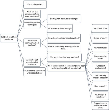
Figure 1. Review framework.
Through this paper, the authors intend to provide a useful guide to researchers and practitioners who are interested in applying deep learning methods to rail track condition monitoring tasks. There are three major contributions of this paper. First, the evolution of deep learning and a collection of relevant deep learning methods provide clear coverage of the relevance, usefulness, and applicability of deep learning methods, which enable fellow researchers to navigate through the usually rather daunting deep learning domain with confidence. Second, a systematic search and review of the application publications proves the relevance of deep learning methods to rail track condition monitoring tasks and provides insights into how such research works are carried out and what potential further studies can be followed up. Third, two illustrative case studies demonstrate practical considerations and aim to motivate wider and more creative adoption of deep learning methods to rail industries. This paper is organized as follows. Section 2 describes a historical overview of deep learning and briefly introduces common deep learning models. Section 3 reviews research adopting deep learning methods for rail track condition monitoring and anomaly detection. Section 4 discusses challenges and opportunities. Section 5 presents case studies applying deep learning to rail anomaly detection and classification while Section 6 concludes the paper.
2. DEEP LEARNING MODELS
2.1. Historical overview of deep learning
We provide a simplified timeline for deep learning and its evolution. Important issues and development at critical junctures are highlighted. A modern definition of deep learning describes a current understanding of the topic. Multiple layers of a deep learning model learn to represent the data with abstractions at multiple levels. The intricate structure of the large input data is discovered through the computations at each layer. Each layer computes its own representation from the representation of its previous layer according to the deep learning model’s internal parameters which are updated using the backpropagation algorithm. Images, video, speech, and audio data can be processed by deep convolutional nets while sequential data such as text and speech by recurrent nets[9]. In the following paragraphs, we examine the journey of deep learning from a single neuron to the current status and hence determine the scope of the following review work.
The McCulloch-Pitts (MCP) neuron proposed in 1943 was the first computational model mimicking the functionality of a biological neuron which marks the start of the era of artificial neural networks. An aggregation of Boolean inputs determines the output through a threshold parameter[10]. The classical perceptron model[11] proposed in 1958 was further refined and analyzed[12] in 1969. The perceptron model brought in the concept of numerical weights to measure the importance of inputs and a mechanism for learning those weights. The model is similar to but more generalized than the MCP neuron as it takes weighted real inputs and the threshold value is learnable. As a single artificial neuron is incapable of implementing some functions such as the XOR logical function, larger networks also have similar limitations which cooled down the artificial neural network development.
The multi-layer perceptron (MLP) was proposed in 1986 where node outputs of hidden layers are calculated using sigmoid function and biogeography based optimization is used to find the weights of the network model[13]. The universal approximation theorem of MLP, proved in 1989, states that, for any given function f(x), there is a backpropagation neural network that can approximately approach the result[14]. The LeNet network was proposed in 1989 to recognize handwritten digits with good performances[15]. In 1991, with the backpropagation neural network, the vanishing gradient problem was discovered, that is back-propagated error signals either shrink rapidly or grow out of bounds in typical deep or recurrent networks because certain activation functions, such as the sigmoid function, take a large input space but have a small output space between 0 and 1[16]. The LSTM model was proposed in 1997[17] and performs well in predicting sequential data. However, since then, neural networks had not been progressing well until 2006. It is worth mentioning that statistical learning theory, a framework for machine learning, blossomed between 1986 and 2006. Methods and models such as decision trees[18], support vector machines (SVM)[19], AdaBoost[20], kernel SVM[21], and random forests[22] were proposed. Graphical models were proposed in 2001 to provide a description framework for various machine learning methods such as SVM, naïve Bayes, and hidden Markov model[23].
Complementary priors were introduced in 2006 to eliminate the vanishing gradient problem that makes inference difficult in densely connected belief nets that have many hidden layers[24]. The rectified linear activation function (ReLU) was introduced in 2011 and became the default activation function of many neural networks. ReLU outputs the input directly if it is positive; otherwise, it is zero. ReLU is effective in tackling the vanishing gradient problems[25].
In 2012, AlexNet, a large deep convolutional neural network, was developed and trained to participate in the ImageNet large scale visual recognition challenge (ILSVRC) for the first time and delivered state-of-the-art results which drew attention from researchers[26]. AlexNet was the pioneer of using the graphics processing unit (GPU) to train the neural network. In the following years, deep learning became more and more popular, the architecture and training methods were improved rapidly, and the hardware advanced quickly and became more powerful. Deep learning has since been adopted by more industries including the railway industry and delivered more meaningful results. This paper focuses on reviewing research works of deep learning applications to rail track condition monitoring since 2013.
2.2. Common deep learning models
Artificial intelligence, machine learning, and deep learning have developed rapidly in recent years. There are many more deep learning networks than one can practically remember. As the resources to learn a particular deep learning method are abundant, we only list some deep learning methods in this section to provide an overview of the techniques available for practitioners and researchers to select and provide brief introductions about the methods. More detailed guides on implementations can be found from the abundance of references available.
The most commonly heard neural network names are probably CNN and RNN. CNN might be noted as ConvNet. The architecture of a CNN was inspired by the organization of the visual cortex and is analogous to that of the connectivity pattern of neurons in the human brain. Individual neurons respond to stimuli only in a restricted region of the visual field known as the receptive field. A collection of such fields overlaps to cover the entire visual area. CNN takes in an input image, assigns importance (learnable weights and biases) to various aspects/objects in the image, and can differentiate one from the other. In RNN, which was derived from feedforward neural networks, nodes are connected to form a directed graph along a temporal sequence to exhibit temporal dynamic behavior. RNN’s internal states (memory) are utilized to process variable-length sequences of inputs. A typical RNN architecture is LSTM which has feedback connections and can process both single data points (such as images) and entire sequences of data (such as speech or video). Applications of CNN and RNN to rail maintenance operations are commonly available, but CNN has been more widely adopted.
There are also some neural network architectures based on CNN with a novel configuration and supporting specific functions and tasks which might give inspirations for the rail maintenance operations. A Siamese neural network, also called a twin neural network, is an artificial neural network that uses the same weights while working in tandem on two different input vectors to calculate similarity scores of output vectors[27]. Figure 2 shows how the CNN layers are positioned to form the architecture of the Siamese neural network.
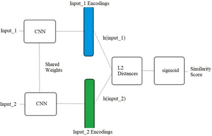
Figure 2. Siamese neural network. CNN: Convolutional neural network
U-Net is a CNN that was developed for biomedical image segmentation. It supplements the usual contracting network by successive layers to increase the output resolutions, where up-sampling operators replace pooling operations[28]. Figure 3 shows how the CNN layers are positioned to form the architecture of the U-Net.
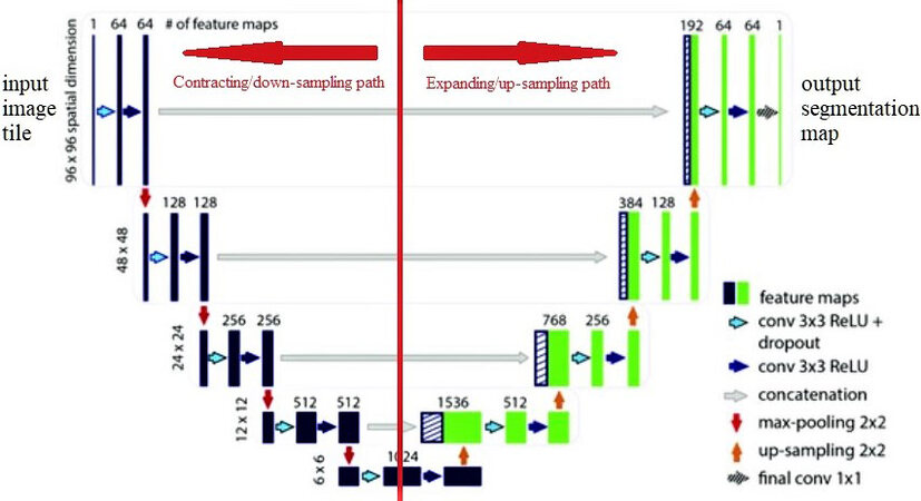
Figure 3. A sample U-Net architecture.
Transfer learning and generative adversarial networks (GANs) are exciting and rapidly changing fields that have been drawing attention from researchers and practitioners in and out of the rail industry. The idea of transfer learning [Figure 4] is that a model developed for a task can be reused as the starting point for a model on another task[29]. Pre-trained models are used as the starting point as transfer learning on both computer vision and natural language processing tasks so that computing and human resources can be preserved and provide a big jump for new deep learning tasks.
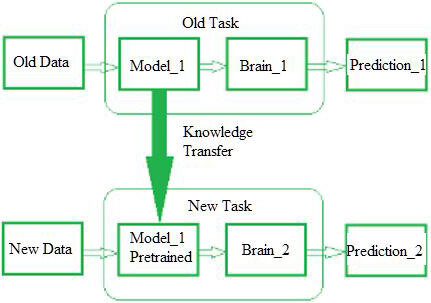
Figure 4. Transfer learning.
Generative modeling is performed to auto-learn and discover the regularities or patterns in input data, and then the model can generate new examples that are plausibly the same as the original dataset[30]. GANs frame the problem with two sub-models: the generator model that is trained to generate new examples, and the discriminator model that tries to classify examples as either real (from the domain) or fake (generated). The two models are adversarially trained together with an objective that the discriminator model cannot distinguish between real and generated inputs. Figure 5 illustrates the main ideas of transfer learning and GANs.
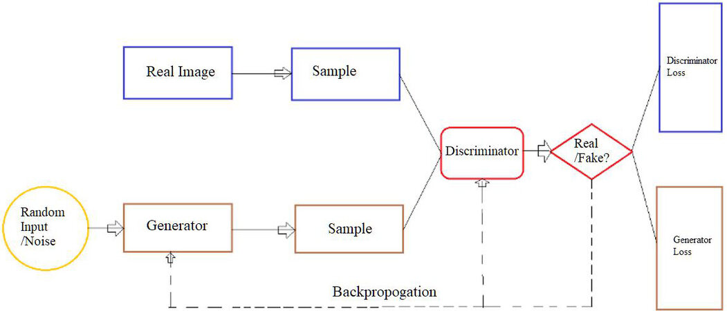
Figure 5. Generative adversarial networks.
There are different deep learning methods suitable for different tasks. The most important problems that humans have been interested in solving with computer vision are image classification, object detection, and segmentation in the increasing order of their difficulty. Rail track anomalies might need to be classified so that appropriate actions can be taken, thus it is an image classification task. A foreign object might need to be located from a rail track image taken, thus it is an object detection task. Sometimes both the types of anomalies and the location of the anomalies need to be identified. It means classification tasks and localization tasks need to be performed concurrently, which is semantic segmentation. Classification networks are created to be invariant to translation and rotation, thus giving no importance to location information, whereas localization involves getting accurate details with respect to the location. Thus, these two tasks are inherently contradictory. Most segmentation algorithms give more importance to localization and thus lose sight of the global context.
For image classification tasks, the following deep learning methods could be adopted:
• LeNet is the earliest pre-trained model used for recognizing handwritten and machine-printed characters and has a simple and straightforward architecture.
• AlexNet consists of eight layers, five convolutional layers and three fully connected layers, features ReLU and overlapping techniques, and allows multiple GPU. The dropout technique is used to prevent overfitting problems while suffering from longer training time. The dropout technique is that, at every training step, the number of interconnecting neurons of a neural network is randomly reduced by a percentage. ZFNet is a classic CNN and was motivated by visualizing intermediate feature layers and the operation of the classifier[31]. It has smaller filters and convolution stride than AlexNet.
• Inception network differs from the CNN classifiers in that it has filters with multiple sizes operating on the same level and concatenated outputs are sent to the next inception module which makes the neural network wider[32].
• GoogLeNet is a 27-layer architecture including nine inception modules that reduce the input images while retaining important spatial information to achieve efficiency. Users can utilize a GoogLeNet network trained on Imagenet with transfer learning instead of implementing or training the network from the scratch.
• ResNet introduces, as shown in Figure 6, an identity shortcut connection that skips one or more layers. The identity mapping layers do nothing to avoid producing higher training error[33]. Pre-activation ResNet makes the optimization easier and reduces the overfitting. RiR (ResNet in ResNet) makes the input with residual stream and transient stream for better accuracy attempts in order to generalize the ResNet block for residual network[34]. Residual networks of residual networks (RoR) proposes to have shortcut connections across a group of residual blocks[35]. On top of this, another level of shortcut connection can exist across a group of “groups of residual blocks”. Wide residual network (WRN) reduces training time but has more parameters as the network widens and it tests plenty of parameters such as the design of the ResNet block including the depth and the widening factor[36].
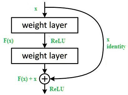
Figure 6. A residual block.
• ResNeXt is a variant to ResNet and looks similar to the inception network as they both follow the split-transform-merge paradigm, but the outputs of different paths are merged by adding them together for ResNeXt instead of depth-concatenated for inception network[37]. ResNeXt architecture’s paths share the same topology. The number of independent paths is introduced as a hyper-parameter cardinality to provide a new way of adjusting the model capacity.
• DenseNet further connects all layers directly with each other for the benefit of shortcut connections[38]. All earlier layers’ feature maps are aggregated with depth-concatenation and passed to subsequent layers. DenseNet is highly parameter-efficient due to feature reuse.
• Network with stochastic depth randomly drops layers during training but uses the full network during testing. The ResNet neural network takes less time in training and is thus more useful for real-world applications[39]. Each layer is randomly dropped with a survival probability during training, and all layers are active and recalibrated according to their survival probabilities during testing time. During training, the input of a residual block flows through both the identity shortcut and the weight layers when it is enabled; otherwise, only it only flows through the identity shortcut.
• VGGNet is a standard deep CNN architecture with 16 and 19 convolutional layers for VGG-16 and VGG-19[40]. The VGG architecture is a well-performing image recognition architecture on many tasks and datasets beyond ImageNet.
• SPPNet is a type of CNN that employs spatial pyramid pooling to remove the fixed-size constraint of the network[41]. An SPP layer is added on top of the last convolutional layer to pool the features and generate fixed-length outputs which are then fed into the fully connected layers or other classifiers with the aim to avoid the need for cropping or warping at the beginning.
• PReLU-Net is a kind of CNN using parameterized ReLUs for activation function and a robust Kaiming initialization scheme to account for non-linear activation functions[42].
• Xception is a 71-layer CNN with an input image size of 299 × 299[43]. The network was trained on more than a million images from the ImageNet database and learned rich feature representations for a wide range of images. Users can load a pre-trained version of the network that can classify images into 1000 object categories.
• MobileNet is a lightweight deep neural network designed for mobile applications of computer vision tasks[44]. As a filter’s depth and spatial dimension can be separated, MobileNet uses depthwise separable convolutions to significantly reduce the number of parameters A depthwise separable convolution is made from depthwise convolution, the channel-wise DK × DK spatial convolution, and pointwise, the 1 × 1 convolution to change the dimension.
• FractalNet is a type of CNN that uses a fractal design instead of residual connections[45]. A simple expansion rule is repeatedly applied to generate deep networks. These networks have structures of truncated fractals and contain interacting subpaths of different lengths. There are no pass-through or residual connections, and every internal signal is transformed before flowing to subsequent layers.
• Both Trimps-Soushen and PolyNet performed very well in the ILSVRC image classification competition. Trimps-Soushen uses the pre-trained models from Inception-v3, Inception-v4, Inception-ResNet-v2, Pre-Activation ResNet-200, and Wide ResNet (WRN-68-2) for classification. PolyNet introduced a building block called PolyInception module formed by adding a polynomial second-order term to increase the accuracy. Then, a very deep PolyNet is composed based on the PolyInception module.
For object detection tasks, the following deep learning methods can be deployed:
• OverFeat is a classic type of CNN architecture, employing convolution, pooling, and fully connected layers[46].
• R-CNN extracts only 2000 regions from the image as region proposals to work with using the selective search algorithm[47]. The CNN extracts the features from the image. The extracted features at the output dense layer are fed into an SVM to classify the presence of the object within that candidate region proposal. For Fast R-CNN, the region proposals are identified from the convolutional feature map generated by the CNN with the input image[48]. The region proposals are then warped into squares and reshaped into a fixed size using a RoI pooling layer before being fed into a fully connected layer. From the RoI feature vector, the class of the proposed region and the offset values for the bounding box are predicted with a softmax layer. Fast R-CNN is faster than R-CNN because the convolution operation is performed only once per image to generate a feature map. Faster R-CNN is similar to Fast R-CNN but much faster. It uses a separate network to predict the region proposals instead of using a selective search algorithm to identify the region proposals on the feature map generated by CNN[49]. An RoI pooling layer then reshapes the predicted region proposals for classifying the image within the proposed region and predicting the offset values for the bounding boxes. Real-time object detection tasks can adopt faster R-CNN.
• DeepID-Net introduces a deformable part-based CNN[50]. A new deformable constrained pooling layer models the deformation of the object parts with geometric constraint and penalty. Besides directly detecting the entire object, it is also crucial to detect object parts which can then support detecting the entire object.
• R-FCN is similar to the logic of R-CNN-based detectors but reduces the amount of work needed for each region proposal to increase the speed[51]. The region-based feature maps can be computed outside each region proposal and are independent of region proposals.
• You only look once (YOLO) algorithm detects objects in real-time using a neural network[52]. Its architecture passes the nxn image once through the fully convolutional neural network and outputs mxm prediction. The YOLO architecture splits the input image into an mxm grid and generates two bounding boxes and associated class probabilities of the boxes for each grid. The bounding boxes could be larger than the grid itself. Differential weights of confidence predictions are adopted for boxes with or without objects during training. The square root of width and height are predicted differently for bounding boxes containing small or large objects. These changes to the loss function enable YOLO to produce better results. YOLOv3 (You Only Look Once, Version 3) was commonly adopted by the studies reviewed here.
• Single Shot multibox Detector (SSD) builds on the VGG-16 architecture while discarding its fully connected layers [Figure 7][53]. The original VGG fully connected layers are replaced with a set of auxiliary convolutional layers (from conv6 onwards) to extract features at multiple scales and progressively decrease the size of the input to each subsequent layer.
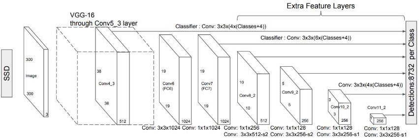
Figure 7. Single Shot multibox Detector architecture.
For semantic segmentation tasks, the following deep learning methods can be adopted:
• FCN uses a CNN to transform image pixels to pixel classes[54]. Instead of image classification or object detection, FCN transforms the height and width of intermediate feature maps back to those of the input image by using the transposed convolutional layer. Thus, the classification output and the input image have a one-to-one correspondence at the pixel level. Therefore, the classification results for the input pixel are held by the channel dimension at its output pixel at the same spatial position.
• DeconvNet gradually deconvolutes and un-pools to obtain its output label map, different from the conventional FCN with possible rough segmentation output label map[55].
• DeepLab applies atrous convolution for up-sampling[56]. Atrous convolution is a shorthand for convolution with up-sampled filters. Filter up-sampling amounts to inserting holes between nonzero filter taps. Atrous convolution allows effectively enlarging the field of view of filters without increasing the number of parameters or the amount of computation. Up-sampling the output of the last convolution layer and computing pixel-wise loss produce the dense prediction.
• ParseNet aggregates the values of each channel feature map’s activations to declare contextual information[57]. These aggregations are then merged to be appended to the final features of the network. This approach is less tiresome than the proposal cum classification approach and avoids unrelated predictions for different pixels under FCN approach.
• DilatedNet uses dilated convolutions, filters with holes, to avoid losing resolution altogether[58]. In this way, the receptive field can grow exponentially while the number of parameters only grows linearly. The front end is based on VGG-16 by replacing the last two pooling layers with dilated convolutions. A context module and a plug-and-play structure are introduced for multi-scale reasoning using a stack of dilated convolutions on a feature map.
• PSPNet utilizes a pyramid parsing module to exploit global context information by aggregating different region-based contexts[59]. A pre-trained CNN with the dilated network strategy is used to extract the feature map, on top of which the pyramid pooling module gathers context information. The final feature map size is one-eighth of the input image. Using a four-level pyramid, the pooling kernels cover the whole, half of, and small portions of the image. They are fused as the global prior, which is then concatenated with the original feature map in the final part. It is followed by a convolution layer to generate the final prediction map. The local and global clues together make the final prediction more reliable.
3. REVIEW OF RAIL TRACK CONDITION MONITORING WITH DEEP LEARNING
The authors systematically searched published peer-reviewed journal articles and papers found in Google Scholar. Combinations of keywords such as “rail”, “surface”, “rail track”, “defect”, and “deep learning” were used as search keys to find research works published in the application of deep learning techniques to rail track condition monitoring and anomaly detection and classification. The review covers work from 2013 to 2021. In total, we identified 62 relevant research publications to review.
The trend over time: a clear increasing trend can be observed of the popularity of deep learning approaches in rail track condition monitoring applications. Table 1 summarizes the findings. The number of papers surged in 2018. Before 2018, machine learning techniques other than deep learning approaches were more widely adopted. The rail industries are adopting deep learning methods with growing interests. An upwards trend of publication number is observed. There is also a gap of a few years from the invention of a deep learning model to its adoption by the rail industry.
Number of papers over time
Regions of study: fourteen regions are represented by the papers identified. Among them, China has the highest number of papers, which indicates the popularity of rail-related research work corresponding to the expanding rail networks across the country. Papers from China surged in 2018 and kept a high number in the following years. Table 2 summarizes the distribution of papers over regions.
Paper distribution over regions
Raw data type: it is observed that 70% of studies used image-type raw data for the deep learning models. Nevertheless, acoustic emission signals[65,71,100,103,108], defectogram[96,109], speed accelerations[98], concatenated vector of curve and numbers[101], current signal[89], maintenance records[80,99], synthetic data from generative model[63], time-frequency measurement data[82], time-series[60], geometry data[87], and vibration signal[119] could all be possible input data sources as well.
Purpose of study: it is observed that detection, classification, and/or localizing rail surface defects including various components (rail, insulator, valves, fasteners, switches, track intrusions, etc.) are the most common purpose of the studies. There are also papers on predicting maintenance time[99] and detecting track geometry elevations[98]. Detection and classification tasks are more common than prediction tasks[60,80,87,99,119].
Adoption of deep learning models: many deep learning models are adopted by researchers. Table 3 summarizes the distribution of deep learning models. CNN is the most popular deep learning model being adopted; however, many researchers created their own structure or divided their tasks into a few stages. CNN has been popular for extracting features and RNN/LSTM has been used for the sequential data type.
Adoption of deep learning models
| Deep learning model | Ref. |
| AlexNet, ResNet | [76] |
| Autoencoder | [89,101] |
| CNN | [61,62,65,68,69,74,75,79,85,94,95,102,108,109] |
| CNN (object detection), RNN (distance estimation) | [93] |
| CNN + YOLOv3 | [117] |
| CNN based self-proposed DFF-Net | [118] |
| CNN based self-proposed FR-Net | [72] |
| CNN to extract feature, only 1 class | [82] |
| CNN, transfer learning | [64] |
| CNN, transfer learning, Bayesian optimization to tune hyperparameters | [100] |
| CNN-LSTM | [87,103,107] |
| Faster R-CNN | [78,88] |
| Faster R-CNN + CNN | [73] |
| FastNet, convolutional network-based | [120] |
| Fine-grained bilinear CNNs model | [70] |
| FCN | [119] |
| GAN for CNN | [115] |
| Inception-ResNet-v2 & CNN | [113] |
| LSTM-RNN | [63,71,99] |
| Mask R-CNN | [121] |
| ML Tree based methods | [80] |
| MobileNetV2, YOLOv3 | [84] |
| Multilayer feedforward neural networks based on multi-valued neurons (MLMVN) | [60] |
| neural network | [96] |
| Point Cloud deep learning | [92] |
| ResNet classifier, DenseNet classifier | [81] |
| ResNet, FCN | [83] |
| Resnet50, transfer learning, Inception, Faster R-CNN | [67] |
| Self-proposed, 2 stage FaultyNet, CNN based | [97] |
| Self-proposed, segment U-Net (CNN based) then detect, progressive | [116] |
| Self-proposed, ShuffleNet-v2 extracts features from the track image, RPN predicts | [86] |
| Siamese convolutional neural network | [66,91] |
| Single Shot multibox Detector (SSD) | [90] |
| SqueezeNet, MobileNetV2 | [111] |
| U-Net to segment | [105] |
| Variational autoencoder | [98] |
| YOLO V3 | [77,104,106,110,114] |
| YOLOv5 detect object; mast R-CNN detect surface defect; ResNet classify fastener state | [112] |
From the summary in Table 3, there are various deep learning methods being adopted in different forms. The effectiveness and the results differ from each other depending on the tasks. It is observed that image is the most popular input data type used for deep learning applications. However, there is a consistent process flow for how to apply the deep learning methods to rail track condition monitoring. First, the image acquisition subsystem (cameras/recording devices) is usually installed on rail engineering maintenance vehicles to capture raw input data. Second, the raw input data are transferred to the image processing subsystem where optional data pre-processing could be performed. Images could be resized, enhanced, have noise removed, or cropped for target areas with image processing techniques. Third, the input data are prepared for the training and testing of deep learning models. Data are labeled accordingly and then randomly assigned for training and testing purposes. Fourth, the selected deep learning model is trained with the training data and validated by the testing data. Depending on the purposes, the deep learning model could perform classification or localization tasks. It is also possible to perform classification and localization concurrently, which is the most common type of task. The feature representations of the input data are always extracted; however, the next steps to deal with the feature vectors differ. It is noted that researchers also proposed their own neural network architectures to replace or complement the existing architectures[72,86,97,116,118]. Fifth, the trained deep learning model is put in production with the trained parameters for real-world applications. Due to the criticality of rail track condition monitoring, redundancy of inspections by human operators could be provided to double confirm the accuracy. Finally, the efficiency and effectiveness of the deep learning models are reviewed and enhanced for improved performances.
Various deep learning methods are reported to produce promising results. With more data available from the rail industry, breakthroughs of deep learning methods, and more advanced and cheaper hardware, deep learning methods will only become more popular and useful for rail track condition monitoring. Deep learning models performed well for feature extraction and data classification tasks. The image processing requirements and the man-made feature extraction efforts are low for deep learning methods, which make the application economical. However, the nature of rail operations causes the distribution of rail track image data to be uneven and extremely disproportional, which could cause class imbalance problems in deep learning applications. The extremely high safety requirement of rail operations and the considerably black-box nature of deep learning models contradict each other and might cause some trust issues, which is demonstrated by the redundancies applied to rail track inspections.
Data pre-processing: removing outliers, normalizing data, and applying image process techniques to enhance the images are common pre-processing techniques. Fourier transforms such as Fast Fourier Transforms and Short Time Fourier Transform have been applied to transform sequential data (e.g., acoustic emission) to 2D spectrograms, which can then be applied to CNN models[65,82,108].
4. DISCUSSIONS
Condition monitoring and anomaly detection and classification are important to a productive rail maintenance operation. There are four main types of maintenance strategies: corrective maintenance, preventive maintenance, proactive maintenance, and predictive maintenance. Deep learning methods can support the maintenance strategies depending on the tasks it performs. For example, detection of a certain type of defect will normally trigger corrective maintenance actions to rectify the rail track. The prediction tasks supported by deep learning methods can be used for predictive maintenance strategies, and they are becoming more and more popular.
Internet of Things (IoT) technologies can be implemented to support rail maintenance operations. Sensor, networking, and application layers in IoT can collect big data, which can then be analyzed by deep learning techniques for application services. In rail track condition monitoring, various types of sensors are being deployed across the rail network to collect data that need enablers such as deep learning techniques to unleash their full potential.
Deep learning methods can be more effective when they can be used in real time in the field by the technicians. Integration of deep learning, IoT, mobile technologies, and edge computing has the potential to develop useful applications that support the daily rail track maintenance operations.
Deep learning models are normally trained with high computing powers. In order for the deep learning models to be used in the field, light deep learning models need to be developed so that less powerful but more accessible devices such as mobile phones can be used with deep learning techniques to support the rail maintenance operations.
Image data have been widely used with useful results. However, they tend to be used in detection and classification, which normally correspond to corrective or preventive maintenance strategies. In order for the industry to advance to predictive maintenance, the causes of defects need to be investigated and corresponding signals can be used for deep learning models’ training and testing. Thus, deep learning application in rail track condition monitoring need to cater to more varieties of data types; for example, the vibration signal is normally a sequential signal and vibration tends to cause wear on the rails over time.
The performance of deep learning models such as accuracy, response time, and precision tend to be influenced by the data used. Therefore, a common dataset of rail tracks will be helpful for researchers to use and validate the performance of deep learning models developed around the world. True performance comparisons could be made as well.
There are always more sections of normal rail tracks than defective sections; therefore, the number of normal track images tend to be much more than the defective ones. When considering the different classes of defects, the number of defect images will be even lower, which can cause class imbalance issues. GAN is a deep learning-based generative model. With the application of GAN to generate more images of defects, the training of deep learning models for detecting and classifying rail defects could be more efficient and accurate.
Transfer learning focuses on storing knowledge gained while solving one problem and applying it to a different but related problem. As rail track condition monitoring task is shared by researchers around the world, a “more” related problem and the knowledge gained will be more useful when it is transferred to another problem but in the same industry. This could be a promising research area for future work.
Reinforcement learning is the training of machine learning models to make a sequence of decisions. The agent learns to achieve a goal in an uncertain, potentially complex environment. This trial-and-error approach suits well the complex situation of deciding when it is the right time to perform the maintenance operations. This research area could generate meaningful results for the industry.
5. ILLUSTRATIVE CASE STUDIES
In this section, we use two application examples to illustrate the implementation of deep learning models to support rail track condition monitoring and rail defect detection and classification.
5.1. Data acquisition and preparations
Data acquisition equipment or devices could be installed on the rail inspection vehicles or passenger trains at different positions. We use rail vision systems here to record videos of the rail tracks for both head and rail checks. Lights are usually required to further enhance the quality of images taken; we use halogen floodlights to support visibility. The train speed might affect the image quality; therefore, a maximum speed may be set. For us, it is 100 km/h. Figure 8 illustrates a typical setup.
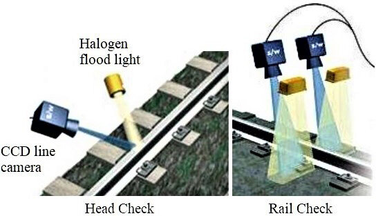
Figure 8. Image acquisition setup.
Various types of input data (image, sound, vibration, etc.) could be adopted for deep learning tasks. For image data, different formats and sizes might be used. Original greyscale images are captured from the rail track videos and then used without segmenting the tracks from the ballast, the sleepers, or other background textures around the rail tracks so as to minimize the image pre-processing efforts and maximize the utility of deep learning models. Pre-processing of input images is optional. Figure 9 shows a sample image that was used for training and test purpose.
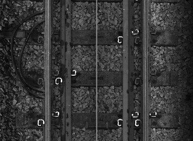
Figure 9. A sample image for training.
We worked with rail maintenance operations staff to describe and label the images according to their properties. Figure 10 shows some sample patterns of “normal”, “corrugation”, “insulated rail joint”, and “weld” images.
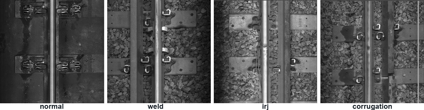
Figure 10. Sample patterns of different classes.
5.2. Deep learning environment configurations
The deep learning experiments were performed on a platform with OS (Windows or Linux) and GPU. Our configurations include Intel Core i7-8700 CPU, Nvidia GeForce RTX 2080 Ti GPU, and 64 GB RAM. Software packages such as Python 3.6, Nvidia CUDA Toolkit, cuDNN, and TensorFlow with GPU support were installed on Windows 10 operating system for our experiments.
5.3. Application 1: CNN
We conducted training and prediction experiments for both anomaly detection and classification purpose. The input images were categorized by the neural network into two output classes for detection tasks and ten output classes for classification tasks. For both tasks, 90% of the image samples were randomly reserved for training while the remaining 10% for testing for every class. In anomaly detection, the distribution of images is comprised of 57% normal images and 43% images with various types of defects. In anomaly classification, there are ten classes in total that are to be classified; their distributions are: 57%, 7%, 2%, 4%, 1%, 1%, 7%, 2%, 17%, and 2%. Input greyscale images were resized to 186 × 256 pixels before being fed into the neural network for training and prediction.
Four convolutional layers, two max-pooling layers, and four fully connected layers were connected for the deep convolutional neural network, and the convolutional kernel size was set as 3 × 3 pixels. We used max-pooling units of size 2 × 2 pixels. ReLU was used as an activation function for convolutional layers. We added a dropout layer as an effective regularization method after max-pooling to reduce overfitting by randomly dropping out nodes during training. After the convolutional and max-pooling layers, we used fully connected layers to perform high-level reasoning in a convolution neural network.
We ran the deep convolutional neural network model for detection and classification tasks separately while keeping the training and testing images the same and only adjusting the number of output classes for the network classifiers at the end of the network. The learning rate of the Adam optimizer was set as 0.001 for training the model. For both the binary classification of detection tasks and the multi-class classification of classification tasks, we counted the number of true positives, true negatives, false positives, and false negatives. The binary classification accuracy was calculated as 87.45% and F1-score as 88.33%. The performance is acceptable and substantially improves the performance of the existing auto-detect method based on image process techniques and man-made feature representations in operation.
5.4. Application 2: Siamese neural network
We conducted training and prediction experiments for classification tasks with four classes of data which comprise normal images and three common types of defects. We used an equal number of images for each class. We created the training data samples for Siamese neural network, which is much easier than the classic convolutional neural network datasets that require images to be labeled. Image samples were randomly chosen from this dataset to form anchor-positive-negative trios. While sampling an image pair, the two images were chosen from the same category with a probability of 0.5 with a corresponding label of y = 0. Similarly, the images were chosen from two different categories with the remaining probability of 0.5 with the label y = 1.
Two identical four-layer convolutional neural networks were used to form the twin structure of the Siamese neural network to perform the identification of rail surface defects. The batch size was 128. The number of epochs was 50. The number of steps per epoch was 5. ReLU was used as an activation function. The neural network optimizer used was Adam. During testing, data of matching pairs and non-matching pairs were formed by randomly selecting images from each of the categories. All combinations, for example, “Normal vs. Defect_1” or “Defect_2 vs. Defect_3”, were tested with 10 pairs and the mean, minimum, and maximum values of test output distance were summarized for analysis. During the testing phase, the images were chosen randomly. These images belonged to a different set of classes that were never shown to the network during training. As described, all combinations of pairwise comparisons were tested with 10 different sample image pairs. The mean Euclidean (L2) distance was computed as the similarity score.
Our experiment results show that, when two test images belong to the same class, their dissimilarity score is smaller than those of images from two different classes. A threshold value can be chosen to determine whether two images are from the same or different classes based on the test similarity scores. We also notice that the threshold value has a decent margin to vary. From our experiments, 82.5% of test images actually from the same class were predicted to be “from the same class”, while 80.8% of test images actually from different classes were predicted to be “from different classes”. The binary classification accuracy was calculated as 81.67% and F1-score as 81.82%. The accuracy level is acceptable to the current rail maintenance operations with the potentials for further improvement.
Both cases can perform rail track condition monitoring and anomaly detection and classifications tasks with deep learning methods with the same dataset. The case studies deal with them in different ways with different deep learning models. Datasets generated from the maintenance operations are put into good use with the deep learning models to improve the rail track maintenance operations. Training of Siamese convolutional neural network was observed to take a shorter time than the classic convolutional neural network approach. The existing hardware setup in the rail operations did not require significant modification. The features extracted by the deep learning models performed better than the approaches of selected man-made features.
6. CONCLUSIONS
This paper presents the importance and criticality of rail track condition monitoring to safe rail operations. We give a brief overview of the historical development of deep learning and list common deep learning models. Deep learning came into the rapid development phase after 2012; therefore, we review the deep learning applications to rail track condition monitoring from 2013 to 2021. The applications are reviewed according to the temporal evolutions, the regional adoptions, the data type, and the deep learning models. We then discuss the potential challenges and research opportunities for applying deep learning to rail track condition monitoring. Two application case studies are shared to illustrate the implementation of deep learning methods in rail track condition monitoring.
DECLARATIONS
AcknowledgmentThis research is part of the project supported by SMRT Corporation Ltd. The opinions, findings, and conclusions or recommendations expressed in this publication are those of the author(s) and do not necessarily reflect those of the company.
Authors’ contributionsInvestigated the research area, reviewed and summarized the literature, wrote and edited the original draft: Ji A
Managed the research activity planning and execution, contributed to the development of ideas according to the research aims: Woo WL, Wong EWL
Performed critical review, commentary and revision, and provided administrative, technical, and material support: Quek YT
Availability of data and materialsNot applicable.
Financial support and sponsorshipNone.
Conflicts of interestAll authors declared that there are no conflicts of interest.
Ethical approval and consent to participateNot applicable.
Consent for publicationNot applicable.
Copyright© The Author(s) 2021.
REFERENCES
1. Cannon DF, Edel K, Grassie SL, Sawley K. Rail defects: an overview. Fatigue Fract Eng M 2003;26:865-86.
2. Track circuit monitoring tool: standardization and deployment at CTA. Available from: http://www.trb.org/Main/Blurbs/177054.aspx [Last accessed on 5 Jan 2022].
3. Rail Defects Handbook. Available from: https://extranet.artc.com.au/docs/eng/track-civil/guidelines/rail/RC2400.pdf [Last accessed on 5 Jan 2022].
4. Dey A, Kurz J, Tenczynski L. Detection and evaluation of rail defects with non-destructive testing methods. Available from: https://www.ndt.net/article/wcndt2016/papers/we1g4.pdf [Last accessed on 5 Jan 2022].
5. Min Y, Xiao B, Dang J, Yue B, Cheng T. Real time detection system for rail surface defects based on machine vision. J Image Video Proc 2018; doi: 10.1186/s13640-017-0241-y.
6. Serin G, Sener B, Ozbayoglu AM, Unver HO. Review of tool condition monitoring in machining and opportunities for deep learning. Int J Adv Manuf Technol 2020;109:953-74.
7. Zhao R, Yan R, Chen Z, Mao K, Wang P, Gao RX. Deep learning and its applications to machine health monitoring. Mech Syst Signal Process 2019;115:213-37.
8. Fu J, Chu J, Guo P, Chen Z. Condition monitoring of wind turbine gearbox bearing based on deep learning model. IEEE Access 2019;7:57078-87.
10. Mcculloch WS, Pitts W. A logical calculus of the ideas immanent in nervous activity. Bull Math Biol 1943;5:115-33.
11. Rosenblatt F. The perceptron: a probabilistic model for information storage and organization in the brain. Psychol Rev 1958;65:386-408.
13. Rodan A, Faris H, Alqatawna J. Optimizing feedforward neural networks using biogeography based optimization for E-mail spam identification. IJCNS 2016;9:19-28.
14. Robert HN. Theory of the backpropagation neural network. Proc 1989 IEEE IJCNN 1989;1:593-605.
15. Lecun Y, Boser B, Denker JS, et al. Backpropagation applied to handwritten zip code recognition. Neural Comput 1989;1:541-51.
16. Hochreiter S. Untersuchungen zu dynamischen neuronalen Netzen. Diploma: Technische Universität München 1991; doi: 10.1515/physiko.17.31.
20. Freund Y, Schapire RE. A decision-theoretic generalization of on-line learning and an application to boosting. J Comput Syst Sci 1997;55:119-39.
21. Cristianini N, Scholkopf B. Support vector machines and kernel methods: the new generation of learning machines. Ai Magazine 2002;23:31.
23. Murphy K. An introduction to graphical models. Rap tech 2001;96:1-19.
24. Hinton GE, Osindero S, Teh YW. A fast learning algorithm for deep belief nets. Neural Comput 2006;18:1527-54.
25. Glorot X, Bordes A, Bengio Y. Deep sparse rectifier neural networks. Proceedings of the 14th International Conference on Artificial Intelligence and Statistics (AISTATS); Fort Lauderdale, FL, USA. 2011. p. 315-23.
26. Krizhevsky A, Sutskever I, Hinton GE. ImageNet classification with deep convolutional neural networks. Commun ACM 2017;60:84-90.
27. Koch G, Zemel R, Salakhutdinov R. Siamese neural networks for one-shot image recognition. Proceedings of the 32nd International Conference on Machine Learning; Lille, France. 2015.
28. Ronneberger O, Fischer P, Brox T. U-Net: convolutional networks for biomedical image segmentation. In: Navab N, Hornegger J, Wells WM, Frangi AF, editors. Medical image computing and computer-assisted intervention - MICCAI 2015. Cham: Springer International Publishing; 2015. p. 234-41.
29. Tan C, Sun F, Kong T, Zhang W, Yang C, Liu C. A survey on deep transfer learning. In: Kůrková V, Manolopoulos Y, Hammer B, Iliadis L, Maglogiannis I, editors. Artificial neural networks and machine learning - ICANN 2018. Cham: Springer; 2008. p. 270-9.
30. Goodfellow I, Pouget-abadie J, Mirza M, et al. Generative adversarial networks. Commun ACM 2020;63:139-44.
31. Zeiler MD, Fergus R. Visualizing and understanding convolutional networks. In: Fleet D, Pajdla T, Schiele B, Tuytelaars T, editors. Computer Vision - ECCV 2014. Cham: Springer International Publishing; 2014. p. 818-33.
32. Szegedy C, Liu W, Jia Y, et al. Going deeper with convolutions. Proceedings of 2015 IEEE Conference on Computer Vision and Pattern Recognition (CVPR); 2015 Jun 7-12; Boston, MA. IEEE; 2005. p. 1-9.
33. He K, Zhang X, Ren S, Sun J. Deep residual learning for image recognition. Proceedings of 2016 IEEE Conference on Computer Vision and Pattern Recognition (CVPR); 2016 Jun 27-30; Las Vegas, NV, USA. IEEE; 2016. p. 770-8.
34. Targ S, Almeida D, Lyman K. Resnet in resnet: generalizing residual architectures. arXiv preprint arXiv:1603.08029.
35. Zhang K, Sun M, Han TX, Yuan X, Guo L, Liu T. Residual networks of residual networks: multilevel residual networks. IEEE Trans Circuits Syst Video Technol 2018;28:1303-14.
36. Zagoruyko S, Komodakis N. Wide residual networks. arXiv preprint arXiv:1605.07146.
37. Xie S, Girshick R, Dollár P, Tu Z, He K. Aggregated residual transformations for deep neural networks. Proceedings of 2017 IEEE Conference on Computer Vision and Pattern Recognition (CVPR); 2017 Jul 21-26; Honolulu, HI, USA. IEEE; 2017. p. 5987-95.
38. Huang G, Liu Z, Van Der Maaten L, Weinberger KQ. Densely connected convolutional networks. Proceedings of 2017 IEEE Conference on Computer Vision and Pattern Recognition (CVPR); 2017 Jul 21-26; Honolulu, HI, USA. IEEE; 2017. p. 2261-9.
39. Huang G, Sun Y, Liu Z, Sedra D, Weinberger KQ. Deep networks with stochastic depth. In: Leibe B, Matas J, Sebe N, Welling M, editors. Computer vision - ECCV 2016. Cham: Springer International Publishing; 2016. p. 646-61.
40. Simonyan K, Zisserman A. Very deep convolutional networks for large-scale image recognition. arXiv preprint arXiv:1409.1556.
41. He K, Zhang X, Ren S, Sun J. Spatial pyramid pooling in deep convolutional networks for visual recognition. IEEE Trans Pattern Anal Mach Intell 2015;37:1904-16.
42. He K, Zhang X, Ren S, Sun J. Delving deep into rectifiers: surpassing human-level performance on imagenet classification. Proceedings of 2015 IEEE International Conference on Computer Vision (ICCV); 2015 Dec 7-13; Santiago, Chile. IEEE; 2015. p. 1026-34.
43. Chollet F. Xception: deep learning with depthwise separable convolutions. Proceedings of 2017 IEEE Conference on Computer Vision and Pattern Recognition (CVPR); 2017 Jul 21-26; Honolulu, HI, USA. IEEE; 2017. p. 1800-7.
44. Howard AG, Zhu M, Chen B, et al. Mobilenets: efficient convolutional neural networks for mobile vision applications. arXiv preprint arXiv:1704.04861.
45. Larsson G, Maire M, Shakhnarovich G. Fractalnet: ultra-deep neural networks without residuals. arXiv preprint arXiv:1605.07648.
46. Sermanet P, Eigen D, Zhang X, Mathieu M, Fergus R, LeCun Y. Overfeat: integrated recognition, localization and detection using convolutional networks. arXiv preprint arXiv:1312.6229.
47. Girshick R, Donahue J, Darrell T, Malik J. Rich feature hierarchies for accurate object detection and semantic segmentation. Proceedings of 2014 IEEE Conference on Computer Vision and Pattern Recognition; 2014 Jun 23-28; Columbus, OH, USA. IEEE; 2014. p. 580-7.
48. Girshick R. Fast R-CNN. Proceedings of 2015 IEEE International Conference on Computer Vision (ICCV); 2015 Dec 7-13; Santiago, Chile. IEEE; 2015. p. 1440-8.
49. Ren S, He K, Girshick R, Sun J. Faster R-CNN: towards real-time object detection with region proposal networks. IEEE Trans Pattern Anal Mach Intell 2017;39:1137-49.
50. Ouyang W, Zeng X, Wang X, et al. DeepID-Net: deformable deep convolutional neural networks for object detection. IEEE Trans Pattern Anal Mach Intell 2017;39:1320-34.
51. Dai J, Li Y, He K, Sun J. R-fcn: object detection via region-based fully convolutional networks. Available from: https://arxiv.org/pdf/1605.06409.pdf [Last accessed on 5 Jan 2022].
52. Redmon J, Divvala S, Girshick R, Farhadi A. You only look once: unified, real-time object detection. Proceedings of 2016 IEEE Conference on Computer Vision and Pattern Recognition (CVPR); 2016 Jun 27-30; Las Vegas, NV, USA. IEEE; 2016. p. 779-88.
53. Liu W, Anguelov D, Erhan D, et al. SSD: Single Shot MultiBox Detector. In: Leibe B, Matas J, Sebe N, Welling M, editors. Computer vision - ECCV 2016. Cham: Springer International Publishing; 2016. p. 21-37.
54. Shelhamer E, Long J, Darrell T. Fully convolutional networks for semantic segmentation. IEEE Trans Pattern Anal Mach Intell 2017;39:640-51.
55. Noh H, Hong S, Han B. Learning deconvolution network for semantic segmentation. Proceedings of 2015 IEEE International Conference on Computer Vision (ICCV); 2015 Dec 7-13; Santiago, Chile. IEEE; 2015. p. 1520-8.
56. Chen LC, Papandreou G, Kokkinos I, Murphy K, Yuille AL. DeepLab: semantic image segmentation with deep convolutional nets, atrous convolution, and fully connected CRFs. IEEE Trans Pattern Anal Mach Intell 2018;40:834-48.
57. Liu W, Rabinovich A, Berg AC. Parsenet: looking wider to see better. arXiv preprint arXiv:1506.04579.
58. Yu F, Koltun V. Multi-scale context aggregation by dilated convolutions. arXiv preprint arXiv:1511.07122.
59. Zhao H, Shi J, Qi X, Wang X, Jia J. Pyramid scene parsing network. Proceedings of 2017 IEEE Conference on Computer Vision and Pattern Recognition (CVPR); 2017 Jul 21-26; Honolulu, HI, USA. IEEE; 2017. p. 6230-9.
60. Fink O, Zio E, Weidmann U. Predicting component reliability and level of degradation with complex-valued neural networks. Reliability Engineering & System Safety 2014;121:198-206.
61. Giben X, Patel VM, Chellappa R. Material classification and semantic segmentation of railway track images with deep convolutional neural networks. Proceedings of 2015 IEEE International Conference on Image Processing (ICIP); 2015 Sep 27-30; Quebec City, QC, Canada. IEEE; 2015. p. 621-5.
62. Faghih-Roohi S, Hajizadeh S, Núnez A, Babuska R, De Schutter B. Deep convolutional neural networks for detection of rail surface defects. Proceedings of 2016 International joint conference on neural networks (IJCNN); 2016 Jul 24-29; Vancouver, BC, Canada. IEEE; 2016. p. 2584-9.
63. Bruin T, Verbert K, Babuska R. Railway track circuit fault diagnosis using recurrent neural networks. IEEE Trans Neural Netw Learn Syst 2017;28:523-33.
64. Gibert X, Patel VM, Chellappa R. Deep multitask learning for railway track inspection. IEEE Trans Intell Transport Syst 2017;18:153-64.
65. Zhang X, Wang K, Wang Y, Shen Y, Hu H. An improved method of rail health monitoring based on CNN and multiple acoustic emission events. Proceedings of 2017 IEEE International Instrumentation and Measurement Technology Conference (I2MTC); 2017 May 22-25; Turin, Italy. IEEE; 2017. p. 1-6.
66. Rao DJ, Mittal S, Ritika S. Siamese neural networks for one-shot detection of railway track switches. arXiv preprint arXiv:1712.08036.
67. Mittal S, Rao D. Vision based railway track monitoring using deep learning. arXiv preprint arXiv:1711.06423.
68. Santur Y, Karaköse M, Akin E. A new rail inspection method based on deep learning using laser cameras. Proceedings of 2017 International Artificial Intelligence and Data Processing Symposium (IDAP); 2017 Sep 16-17; Malatya, Turkey. IEEE; 2017. p. 1-6.
69. Santur Y, Karaköse M, Akin E. An adaptive fault diagnosis approach using pipeline implementation for railway inspection. Turk J Elec Eng & Comp Sci 2018;26:987-98.
70. Huang H, Xu J, Zhang J, Wu Q, Kirsch C. Railway infrastructure defects recognition using fine-grained deep convolutional neural networks. Proceedings of 2018 Digital Image Computing: Techniques and Applications (DICTA); 2018 Dec 10-13; Canberra, ACT, Australia. IEEE; 2018. p. 1-8.
71. Zhang X, Zou Z, Wang K, et al. A new rail crack detection method using LSTM network for actual application based on AE technology. Appl Acoust 2018;142:78-86.
72. Ye T, Wang B, Song P, Li J. Automatic railway traffic object detection system using feature fusion refine neural network under shunting mode. Sensors (Basel) 2018;18:1916.
73. Kang G, Gao S, Yu L, Zhang D. Deep architecture for high-speed railway insulator surface defect detection: denoising autoencoder with multitask learning. IEEE Trans Instrum Meas 2019;68:2679-90.
74. Liang Z, Zhang H, Liu L, He Z, Zheng K. Defect detection of rail surface with deep convolutional neural networks. Proceedings of 2018 13th World Congress on Intelligent Control and Automation (WCICA); 2018 Jul 4-8; Changsha, China. IEEE; 2018. p. 1317-22.
75. Shang L, Yang Q, Wang J, Li S, Lei W. Detection of rail surface defects based on CNN image recognition and classification. Proceedings of 2018 20th International Conference on Advanced Communication Technology (ICACT); 2018 Feb 11-14; Chuncheon, Korea (South). IEEE; 2018. p. 45-51.
76. Wang S, Dai P, Du X, Gu Z, Ma Y. Rail fastener automatic recognition method in complex background. Proceedings of Tenth International Conference on Digital Image Processing (ICDIP 2018); 2018 Aug 9; Shanghai, China. International Society for Optics and Photonics; 2018. p. 1080625.
77. Yanan S, Hui Z, Li L, Hang Z. Rail surface defect detection method based on yolov3 deep learning networks. Proceedings of 2018 Chinese Automation Congress (CAC); 2018 Nov 30-Dec 2; Xi’an, China. IEEE; 2018. p. 1563-8.2
78. Xu X, Lei Y, Yang F. Railway subgrade defect automatic recognition method based on improved faster R-CNN. Sci Programming 2018;2018:1-12.
79. Jamshidi A, Hajizadeh S, Su Z, et al. A decision support approach for condition-based maintenance of rails based on big data analysis. Transp Res Part C Emerg Technol 2018;95:185-206.
80. Bukhsh Z, Saeed A, Stipanovic I, Doree AG. Predictive maintenance using tree-based classification techniques: a case of railway switches. Transp Res Part C Emerg Technol 2019;101:35-54.
81. James A, Jie W, Xulei Y, et al. Tracknet - a deep learning based fault detection for railway track inspection. Proceedings of 2018 International Conference on Intelligent Rail Transportation (ICIRT); 2018 Dec 12-14; Singapore. IEEE; 2018. p. 1-5.
82. Peng X, Jin X. Rail suspension system fault detection using deep semi-supervised feature extraction with one-class data. PHM_CONF 2018; doi: 10.36001/phmconf.2018.v10i1.546.
83. Sun Y, Liu Y, Yang C. Railway joint detection using deep convolutional neural networks. Proceedings of 2019 IEEE 15th International Conference on Automation Science and Engineering (CASE); 2019 Aug 22-26; Vancouver, BC, Canada. IEEE; 2019. p. 235-40.
84. Yuan H, Chen H, Liu S, Lin J, Luo X. A deep convolutional neural network for detection of rail surface defect. Proceedings of 2019 IEEE Vehicle Power and Propulsion Conference (VPPC); 2019 Oct 14-17; Hanoi, Vietnam. IEEE; 2019. p. 1-4.
85. Wang Y, Zhu L, Yu Z, Guo B. An adaptive track segmentation algorithm for a railway intrusion detection system. Sensors (Basel) 2019;19:2594.
86. Dong B, Li Q, Wang J, Huang W, Dai P, Wang S. An end-to-end abnormal fastener detection method based on data synthesis. Proceedings of 2019 IEEE 31st International Conference on Tools with Artificial Intelligence (ICTAI); 2019 Nov 4-6; Portland, OR, USA. IEEE; 2019. p. 149-56.
87. Ma S, Gao L, Liu X, Lin J. Deep learning for track quality evaluation of high-speed railway based on vehicle-body vibration prediction. IEEE Access 2019;7:185099-107.
88. Jin X, Wang Y, Zhang H, et al. DM-RIS: deep multimodel rail inspection system with improved MRF-GMM and CNN. IEEE Trans Instrum Meas 2020;69:1051-65.
89. Li Z, Yin Z, Tang T, Gao C. Fault diagnosis of railway point machines using the locally connected autoencoder. Appl Sci 2019;9:5139.
90. Guo B, Shi J, Zhu L, Yu Z. High-speed railway clearance intrusion detection with improved SSD network. Appl Sci 2019;9:2981.
91. Liu J, Huang Y, Zou Q, et al. Learning visual similarity for inspecting defective railway fasteners. IEEE Sensors J 2019;19:6844-57.
92. Cui H, Li J, Hu Q, Mao Q. Real-time inspection system for ballast railway fasteners based on point cloud deep learning. IEEE Access 2020;8:61604-14.
93. Haseeb M, Ristić-Durrant D, Gräser A. A deep learning based autonomous distance estimation and tracking of multiple objects for improvement in safety and security in railways. Available from: https://www.bmvc2019.org/wp-content/ODRSS2019/ODRSS2019_P_5_Haseeb.pdf [Last accessed on 5 Jan 2022].
94. Chen SX, Ni YQ, Liu JC, Yao N. Deep learning-based data anomaly detection in rail track inspection. Proceedings of 12th International Workshop on Structural Health Monitoring: Enabling Intelligent Life-Cycle Health Management for Industry Internet of Things (IIOT); 2019; Stanford, USA. DEStech Publications Inc.; 2019. p. 3235-42.
95. Jang J, Shin M, Lim S, Park J, Kim J, Paik J. Intelligent image-based railway inspection system using deep learning-based object detection and weber contrast-based image comparison. Sensors 2019;19:4738.
96. Kuzmin EV, Gorbunov OE, Plotnikov PO, Tyukin VA, Bashkin VA. Application of neural networks for recognizing rail structural elements in magnetic and eddy current defectograms. Aut Control Comp Sci 2019;53:628-37.
97. Pahwa RS, Chao J, Paul J, et al. Faultnet: faulty rail-valves detection using deep learning and computer vision. Proceedings of 2019 IEEE Intelligent Transportation Systems Conference (ITSC); 2019 Oct 27-30; Auckland, New Zealand. IEEE; 2019. p. 559-66.
98. Liu J, Wei Y, Bergés M, Bielak J, Garrett Jr JH, Noh H. Detecting anomalies in longitudinal elevation of track geometry using train dynamic responses via a variational autoencoder. Proceedings of Sensors and Smart Structures Technologies for Civil, Mechanical, and Aerospace Systems 2019; 2019 Mar 27; Denver, CO, USA. International Society for Optics and Photonics; 2019. p. 109701B.
99. Wang Q, Bu S, He Z. Achieving predictive and proactive maintenance for high-speed railway power equipment with LSTM-RNN. IEEE Trans Ind Inf 2020;16:6509-17.
100. Li D, Wang Y, Yan W, Ren W. Acoustic emission wave classification for rail crack monitoring based on synchrosqueezed wavelet transform and multi-branch convolutional neural network. Struct Health Monit 2021;20:1563-82.
101. Guo Z, Wan Y, Ye H. An unsupervised fault-detection method for railway turnouts. IEEE Trans Instrum Meas 2020;69:8881-901.
102. Zhan Y, Dai X, Yang E, Wang KC. Convolutional neural network for detecting railway fastener defects using a developed 3D laser system. Int J Rail Transp 2021;9:424-44.
103. Li Z, Zhang J, Wang M, Zhong Y, Peng F. Fiber distributed acoustic sensing using convolutional long short-term memory network: a field test on high-speed railway intrusion detection. Opt Express 2020;28:2925-38.
104. Wei X, Wei D, Suo D, Jia L, Li Y. Multi-target defect identification for railway track line based on image processing and improved YOLOv3 model. IEEE Access 2020;8:61973-88.
105. Lu J, Liang B, Lei Q, et al. SCueU-Net: efficient damage detection method for railway rail. IEEE Access 2020;8:125109-20.
106. Zheng Y, Wu S, Liu D, Wei R, Li S, Tu Z. Sleeper defect detection based on improved YOLO V3 algorithm. Proceedings of 2020 15th IEEE Conference on Industrial Electronics and Applications (ICIEA); 2020 Nov 9-13; Kristiansand, Norway. IEEE; 2020. p. 955-60.
107. Zhang D, Song K, Wang Q, He Y, Wen X, Yan Y. Two deep learning networks for rail surface defect inspection of limited samples with line-level label. IEEE Trans Ind Inf 2021;17:6731-41.
108. Chen S, Zhou L, Ni Y, Liu X. An acoustic-homologous transfer learning approach for acoustic emission-based rail condition evaluation. Struct Health Monit 2021;20:2161-81.
109. Kuzmin EV, Gorbunov OE, Plotnikov PO, Tyukin VA, Bashkin VA. Application of convolutional neural networks for recognizing long structural elements of rails in eddy-current defectograms. Model anal inf sist 2020;27:316-29.
110. Liu Y, Sun X, Pang JHL. (, March). A YOLOv3-based deep learning application research for condition monitoring of rail thermite welded joints. Proceedings of the 2020 2nd International Conference on Image, Video and Signal Processing; 2020 Mar; New York, NY, USA. Association for Computing Machinery; 2020. p. 33-8.
111. Aydin I, Akin E, Karakose M. Defect classification based on deep features for railway tracks in sustainable transportation. Appl Soft Comput 2021;111:107706.
112. Zheng D, Li L, Zheng S, et al. A defect detection method for rail surface and fasteners based on deep convolutional neural network. Comput Intell Neurosci 2021;2021:2565500.
113. Wang W, Hu W, Wang W, et al. Automated crack severity level detection and classification for ballastless track slab using deep convolutional neural network. Autom Constr 2021;124:103484.
114. Chen Z, Wang Q, Yang K, et al. Deep learning for the detection and recognition of rail defects in ultrasound B-scan images. Transp Res Rec 2021;2675:888-901.
115. Liu J, Ma Z, Qiu Y, Ni X, Shi B, Liu H. Four discriminator cycle-consistent adversarial network for improving railway defective fastener inspection. IEEE Trans Intell Transport Syst 2021; doi: 10.1109/tits.2021.3095167.
116. Wu Y, Qin Y, Qian Y, Guo F, Wang Z, Jia L. Hybrid deep learning architecture for rail surface segmentation and surface defect detection. Computer aided Civil Eng 2022;37:227-44.
117. Wan Z, Chen S. Railway tracks defects detection based on deep convolution neural networks. In: Liang Q, Wang W, Mu J, Liu X, Na Z, Cai X, editors. Artificial intelligence in China. Singapore: Springer; 2021. p. 119-29.
118. Ye T, Zhang X, Zhang Y, Liu J. Railway traffic object detection using differential feature fusion convolution neural network. IEEE Trans Intell Transport Syst 2021;22:1375-87.
119. Chen M, Zhai W, Zhu S, Xu L, Sun Y. Vibration-based damage detection of rail fastener using fully convolutional networks. Veh Syst Dyn 2021; doi: 10.1080/00423114.2021.1896010.
120. Tai JJ, Innocente MS, Mehmood O. FasteNet: a fast railway fastener detector. In: Yang X, Sherratt S, Dey N, Joshi A, editors. Proceedings of Sixth International Congress on Information and Communication Technology. Singapore: Springer; 2022. p. 767-77.
Cite This Article
Export citation file: BibTeX | RIS
OAE Style
Ji A, Woo WL, Wong EWL, Quek YT. Rail track condition monitoring: a review on deep learning approaches. Intell Robot 2021;1(2):151-75. http://dx.doi.org/10.20517/ir.2021.14
AMA Style
Ji A, Woo WL, Wong EWL, Quek YT. Rail track condition monitoring: a review on deep learning approaches. Intelligence & Robotics. 2021; 1(2): 151-75. http://dx.doi.org/10.20517/ir.2021.14
Chicago/Turabian Style
Ji, Albert, Wai Lok Woo, Eugene Wai Leong Wong, Yang Thee Quek. 2021. "Rail track condition monitoring: a review on deep learning approaches" Intelligence & Robotics. 1, no.2: 151-75. http://dx.doi.org/10.20517/ir.2021.14
ACS Style
Ji, A.; Woo WL.; Wong EWL.; Quek YT. Rail track condition monitoring: a review on deep learning approaches. Intell. Robot. 2021, 1, 151-75. http://dx.doi.org/10.20517/ir.2021.14
About This Article
Special Issue
Copyright

Data & Comments
Data


 Cite This Article 34 clicks

 Like This Article 37
likes
Like This Article 37
likes


Comments
Comments must be written in English. Spam, offensive content, impersonation, and private information will not be permitted. If any comment is reported and identified as inappropriate content by OAE staff, the comment will be removed without notice. If you have any queries or need any help, please contact us at support@oaepublish.com.