
A review of causality-based fairness machine learning

Abstract
With the wide application of machine learning driven automated decisions (e.g., education, loan approval, and hiring) in daily life, it is critical to address the problem of discriminatory behavior toward certain individuals or groups. Early studies focused on defining the correlation/association-based notions, such as statistical parity, equalized odds, etc. However, recent studies reflect that it is necessary to use causality to address the problem of fairness. This review provides an exhaustive overview of notions and methods for detecting and eliminating algorithmic discrimination from a causality perspective. The review begins by introducing the common causality-based definitions and measures for fairness. We then review causality-based fairness-enhancing methods from the perspective of pre-processing, in-processing and post-processing mechanisms, and conduct a comprehensive analysis of the advantages, disadvantages, and applicability of these mechanisms. In addition, this review also examines other domains where researchers have observed unfair outcomes and the ways they have tried to address them. There are still many challenges that hinder the practical application of causality-based fairness notions, specifically the difficulty of acquiring causal graphs and identifiability of causal effects. One of the main purposes of this review is to spark more researchers to tackle these challenges in the near future.
Keywords
1. INTRODUCTION
Artificial intelligence (AI) techniques are widely applied in various fields to assist people in decision-making, such as hiring [1, 2], loans [3, 4], education [5], criminal risk assessment [6], etc. The motivation for using machine learning models is that they can mine hidden laws and useful information from data with huge volumes and various structures more quickly and effectively than human beings. Most importantly, people often mix personal emotions when making decisions, making their decisions unfavorable to certain groups. It is canonically believed that the decisions made by automatic decision-making systems are more objective, and, thus, there will be no discrimination against specific groups or individuals. However, this assumption cannot always be met. Due to the biased training data and inherent bias of adopted models, machine learning models are not always as neutral as people expect.
Since many automated systems driven by AI techniques can significantly impact people's lives, it is important to eliminate discrimination embedded in the AI models so that fair decisions are made with their assistance. Indeed, in recent years, fairness issues of AI models have been receiving wide attention. For example, automated resume screening systems often give biased evaluations based on traits beyond the control of candidates (e.g., gender and race), which may not only discriminate against job applicants with certain characteristics but also cost employers by missing out on good employees. Early research on achieving fairness of algorithms focused on statistical correlation and developed many correlation-based fairness notions (e.g., predictive parity [7], statistical parity [8], and equalized odds [9]), which primarily focus on discovering the discrepancy of statistical metrics between individuals or sub-populations. However, correlation-based fairness notions fail to detect discrimination in algorithms in some cases and cannot explain the causes of discrimination, since they do not take into account the mechanism by which the data are generated. A classic example is Simpson's paradox [10], where the statistical conclusions are drawn from the sub-populations and the whole population can be different. On the other hand, discrimination claims usually require demonstrating causal relationships between sensitive attributes and questionable decisions, instead of the association or correlation between the sensitive attributes and decisions.
Consider the example of the graduate admissions at University of California, Berkeley in 1973, which confirms the importance of developing causal perspective admission to detect and eliminate discrimination. From the statistical results of historical data, roughly 44% of all men who applied were admitted, compared to 35% of women who applied. Then, a flawed conclusion may be drawn with the support of the difference in admission rates between males and females. That is, there exists discrimination towards women for their graduate admission. After an in-depth examination of this case, there is no wrongdoing by the educational institution, but a larger proportion of women applied to the most competitive departments, causing a lower admission rate than men. However, the question of discrimination is far from resolved, e.g., there is no way of knowing why women tended to apply to more competitive departments from the available data alone. Therefore, it is helpful to detect discrimination and interpret the sources of discrimination by understanding the data generating mechanism, namely the causality behind the problem of discrimination. In addition, causal models can be regarded as a mechanism to integrate scientific knowledge and exchange credible assumptions to draw credible conclusions. For this admission case, it seems that, due to women's socialization and education, they tend to toward fields of studies that are generally crowded. Therefore, it is necessary to explore the causal structure of the problem. Fortunately, more and more researchers have paid attention to detecting and eliminating discrimination from the perspective of causality, and various fairness concepts and fairness-enhancing methods based on causality have been proposed.
Compared with the fairness notions based on correlation, causality-based fairness notions and methods take additional consideration of the knowledge that reflects the causal structure of the problem. This knowledge reveals the mechanism of data generation and is helpful for us to comprehend how the influence of sensitive attributes change spreads in the system, which is conducive to improving the interpretability of model decisions [11-14]. Therefore, causality-based fairness machine learning algorithms help to enhance fairness. However, causality-based fairness approaches still face many challenges, one of which is unidentifiable situations of causal effects [15]. In other words, the causal effect between two variables cannot be uniquely computed from the observational data without extra assumptions.
The previous survey articles offer a high-level summary of technology to eliminate algorithm discrimination, and there is no detailed discussion on specific subareas [16-19]. Wan et al.[20] provided an exhaustive review of the methods of using the in-process mechanism to solve the fairness issues. Makhlouf et al.[21] summarized the advantages and disadvantages of each fairness notion and their suitability, aiming to help us select the fairness notions that are most suitable for a particular scenario. Makhlouf et al.[22] only focused on reviewing the concept of fairness based on causality. Instead of eliminating discrimination from a technical perspective, Wu et al.[23] summarized human-oriented fairness-enhancing methods as a way to explore the role of human beings in addressing algorithmic fairness.
To complement the previous survey papers on fairness-enhancing machine learning, this survey thoroughly reviews the concept of fairness based on causality and summarizes the core ideology behind the causality-based fairness-enhancing approaches. This survey aims to stimulate future exploration of causality-based fairness technology, because of the importance of causal modeling in improving algorithmic fairness. In this survey, the review of the concept and technology of fairness based on causality is conducted in several phases. The survey first reviews causality-based definitions and measures of fairness and summarizes the suitability of these causality-based fairness notions. Next, it provides a comprehensive overview of state-of-the-art methods to achieve fairness based on these causality-based fairness notions. The survey also discusses the practical applications, beyond classification, that the causality-based fairness methods are expected to benefit greatly. Finally, this survey discusses the challenges of eliminating discrimination from a causal perspective, including the acquisition of causal graphs and identifiable issues. It also reviews the efforts for addressing these challenges and summarizes the remaining issues, which provides some assistance to solve these problems for future research. Figure 1 shows the organizational structure of this survey.
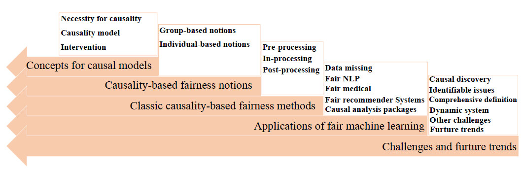
Figure 1. Organizational structure of this paper.
The rest of this survey is structured as follows. Section 2 introduces an example to interpret the importance of causal modeling for addressing fairness issues. Section 3 presents the background of the causal model. Section 4 introduces definitions and measures of causality-based fairness notions and discusses the suitability or applicability of them. Section 5 discusses fairness mechanisms and causality-based fairness approaches, and compares these mechanisms. Section 6 introduces several typical applications of causality-based fairness methods. Section 7 analyzes the challenges and the research trends for applying causality-based fairness-enhancing methods in practical scenarios.
2. THE IMPORTANCE FOR CAUSALITY TO DETECT DISCRIMINATION: AN EXAMPLE
The importance of applying causal analysis to discrimination discovery is explored in this section. Consider a simple example that is inspired by a legal dispute about religious discrimination in recruitment [24]. To keep the situation simple, assuming that a company takes the religious belief
Assume also that the proportions of applicants with faith are equal to those without religious beliefs, and the proportions of applicants with high education are the same as the one with low education, which means that
From such probabilities mentioned above, the company is more likely to hire the applicants without religious beliefs than ones with faith, which indicates that its hiring decisions are unfair. However, this conclusion is wrong, since it only considers the association between religious beliefs and hiring decisions, instead of the causal relationship. In fact, understanding causal mechanisms behind hiring decisions can avoid drawing such wrong conclusions, since it exposes the mechanism of data generation. Through the causal analysis for three variables in the above example, the education level of the individuals is an observable confounder, that is, an individual's educational background influences both his (or her) religious beliefs and hiring decisions made by the company. The higher the education level of individuals, the less willing they are to participate in religious activities. The causal relationships between these variables are shown in Figure 2(a). Based on the causal graph, further causal analysis of hiring decisions of this company is conducted to explore whether it is really discriminatory. In other words, intervention on
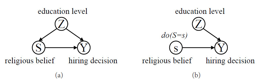
Figure 2. Two causal graphs for the hiring decision system. (a) A causal graph of the hiring decision system, where
These values confirm that the hiring decisions made by the company do not discriminate against applicants with religious beliefs. Therefore, it is critical to conduct a causal analysis of the problem, since understanding the causal mechanisms behind the problem can not only help to detect discrimination but also help to interpret the sources of discrimination.
3. PRELIMINARIES AND NOTATION
In this review, an attribute is denoted by an uppercase letter, e.g.,
One of the most popular causal model frameworks is Pearl's Structural Causal Model (SCM) [10]. A structural causal model
1.
2.
3.
4.
A causal model
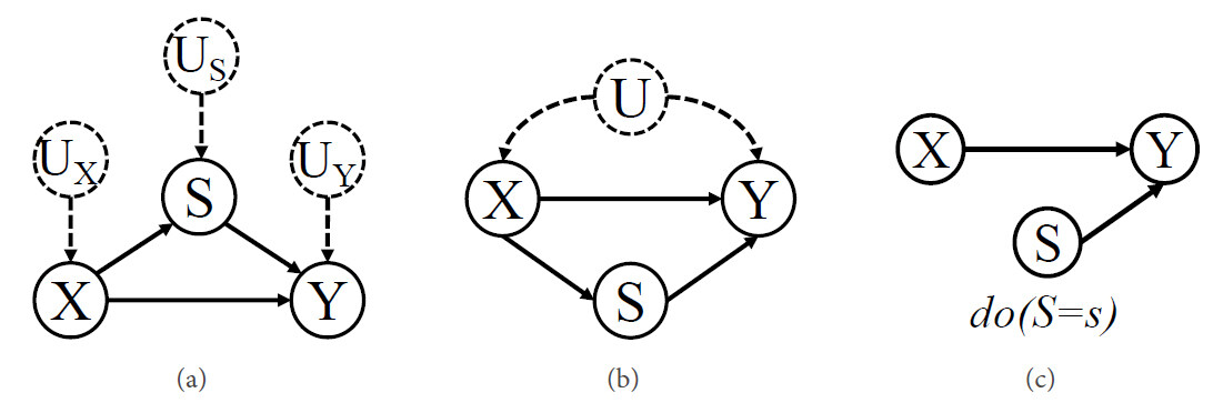
Figure 3. (a) An example causal graph based on Markovian assumption; (b) a causal graph based on semi-Markovian assumption; and (c) a causal graph after performing an intervention on
An intervention simulates the physical interventions that force some variable
Causality-based fairness notions aim to tell whether the outcome of a decision made by the AI decision model is discriminative, which are expressed by interventional and counterfactual probability distributions. The application of the causality-based fairness notions not only requires a dataset
4. CAUSALITY-BASED FAIRNESS NOTIONS
Pearl defined the causality as three rungs: correlation, intervention, and counterfactual [25]. The first rung (correlation) reflects the ability of observation, which aims to discover the patterns in the environment. The second rung (intervention) reflects the ability of action, which refers to the prediction of the results of deliberate changes to the environment. The third rung (counterfactual) refers to the ability to imagine the counterfactual world and speculate on the causes of the observed phenomena. The second and third rungs aim to expose the root causes of the patterns that we observe. Thus far, many fairness metrics have been proposed and all of them can be placed in such causal rungs. Figure 4 presents categorization of fairness notions. Early definitions of fairness are based on statistical correlations, all of which can be found at the first rung. All causality-based fairness notions can be found at the second and third rungs, each of which considers the mechanism of data generation. Thus, causality-based fairness notions can better reveal the causes of discrimination than statistics-based ones and have been attracting more and more attention.
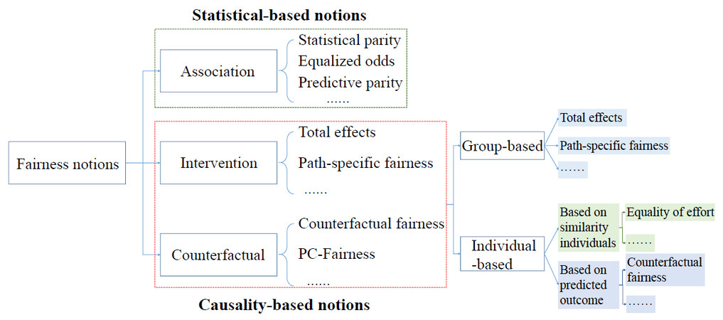
Figure 4. The categorization of fairness notions.
In the real world, the focus of different machine learning tasks is different, and thus, various causality-based fairness notions are proposed to detect discrimination in different scenarios. This section introduces several representative causality-based fairness measurements that quantify fairness from the perspective of groups or individuals, respectively. Without loss of generality, assume that the sensitive attribute
Typical causality-based fairness notions
| Type | Fairness notion | Formulation | Description |
| Group | Total Effect [10] | The causal effects of the value change of the sensitive attribute $$S$$ from $$s^+$$ to $$s^-$$ on decision $$Y=y$$, where the intervention is transmitted along all causal paths and is within the fair threshold $$\tau$$ | |
| Effect of treatment on the treated [10] | The difference between the distribution of $$Y=y$$ had $$S$$ been $$s^+$$ and that of $$Y=y$$ had $$S$$ been $$s^-$$, given that $$S$$ had been observed to be $$s^-$$ | ||
| Path-specific fairness [26, 27] | The causal effects of the value change of the sensitive attribute $$S$$ from $$s^+$$ to $$s^-$$ on decision $$Y=y$$ along specific causal paths, is within the fair threshold $$\tau$$ | ||
| No unresolved discrimination [28] | - | It is satisfied when there is no directed path from sensitive attribute $$S$$ to outcome $$Y$$ allowed, except through a resolving variable | |
| No proxy discrimination [28] | $$P(Y|do(R=r_0)) = P(Y|do(R=r_1))$$ $$\forall r_0, r_1 \in dom(R)$$ | If it is satisfied, there is no path from the sensitive attribute $$S$$ to the outcome $$Y$$ blocked by a proxy variable | |
| Individual | Counterfactual fairness [11] | $$|P(y_{s^+}|{\bf O}={\bf o}, S=s^-)-$$ $$P(y_{s^-}|{\bf O}={\bf o}, S=s^-)| \leq \tau$$ | An outcome $$Y$$ achieves counterfactual fairness towards an individual $$i$$ (i.e., $${\bf O}={\bf o}$$) if the probability of $$Y=y$$ for such individual $$i$$ is the same as the probability of $$Y=y$$ for the same individual, who belongs to a different sensitive group |
| Individual direct discrimination [29] | It is based on situation testing where the causal reasoning is used to define the distance function $$d(i, i')$$ | ||
| Equality of effort [30] | $$\Psi_{G^+}(\gamma) = \Psi_{G^-}(\gamma)$$ where $$\Psi_{G^+}(\gamma) = argmin_{t \in T} {\mathbb{E}[Y_{G^+}^t] \geqslant \gamma}$$ | It detects discrimination by comparing the effort required to reach the same level of outcome of individuals from advantaged and disadvantaged groups who are similar to the target individual | |
| Hybrid | PC-fairness [31] | It is a general fairness formalization for representing various causality-based fairness notions, which is achieved by differently tuning its parameters |
4.1. Group causality-based fairness notions
Group fairness notions aim to discover the difference in outcomes of AI decision models across different groups. The value of an individual's sensitive attribute reflects the group he (or she) belongs to. Considered an example of salary prediction where
4.1.1. Total effect
Before defining total effect (TE) [10], statistical parity (SP) is first introduced, since it is similar to TE but is fundamentally different from TE. SP is a common statistics-based fairness notion, which denotes similar individuals treated similarly regardless of their sensitive attributes. Statistical parity is satisfied if
Intuitively,
TE measures the difference between total causal effect of sensitive attribute
A more complex total effect considers the effect of changes in the sensitive attribute value on the outcome of automated decision making when we already observed the outcome for that individual, which is known as the effect of treatment on the treated (ETT) [10]. This typically involves a counterfactual situation which requires changing the sensitive attribute value of that individual at that time to examine whether the outcome changes or not. ETT can be mathematically formalized using counterfactual quantities as follows:
where
Other fairness notions similar to TE are also proposed. For example, FACT (fair on average causal effect) [32] was proposed to detect discrimination of automated decision making, which is based on potential outcome framework [33, 34]. It considers an outcome
TE and ETT both aim to eliminate the decision bias on all causal paths from
4.1.2. Path-specific fairness
The causal effect of sensitive attribute on the outcome can be divided into direct effect and indirect effect, and it can be deemed fair or discriminatory by an expert. Direct discrimination can be captured by the causal effects of
Figure 5(a) represents the causal graph of a simple example of a toy model of loan decision AI model, where Race is treated as the sensitive attribute and Loan is treated as the decision. Since ZipCode can reflect the information of Race, ZipCode is a proxy for the sensitive attribute, that is to say, ZipCode is a redline attribute. Thus, the causal effects spreading along the path Race
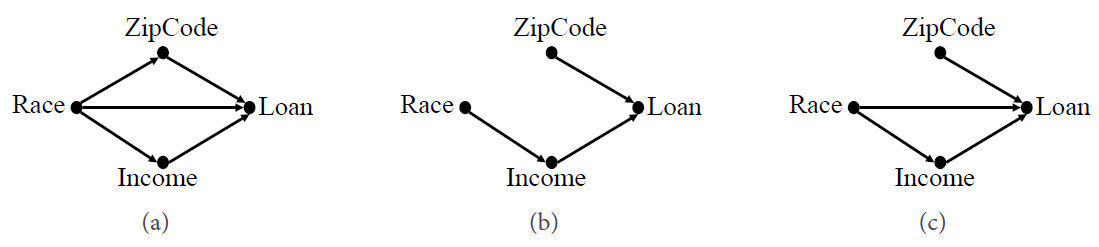
Figure 5. Two alternative graphs for the loan application system. (a) A causal graph of the loan application system, where Race is the sensitive attribute and Loan is the decision. (b) A causal graph of the system after removing unresolved discrimination. (c) A causal graph of the system that is free of proxy discrimination.
Path-specific effect [10] is a fine-grained assessment of causal effects, that is, it can evaluate the causal effect transmitted along certain paths. Thus, it is used to distinguish among direct discrimination, indirect discrimination, and explainable bias. For any set of paths
where
4.1.3. No unresolved/proxy discrimination
No unresolved discrimination [28] is a fairness notion which is based on Pearl's structural causal model framework and aims to detect indirect discrimination. This criterion is satisfied if there is no directed path from the sensitive attribute
Similar to no unresolved discrimination, no proxy discrimination [28] also focuses on indirect discrimination. Given a causal graph, if this criterion is satisfied, the effects of the sensitive attribute
In other words, this notion implies that changing the value of
No unresolved discrimination is a flawed definition of fairness. Specifically, no unresolved discrimination criterion is unable to identify some counterfactual unfair scenarios where some attributes are deemed as the resolved attributes. On the other hand, policy makers and domain professionals should carefully examine the relevance between sensitive variables and other endogenous variables so as to discover all resolving attributes and potential proxies that may lead to discrimination spread.
4.2. Individual causality-based fairness notions
Different from group fairness notions that measure the differences in the outcome of decision models between advantaged groups and disadvantaged ones, individual fairness notions aim to examine whether the outcome of decision models is fair to each individual in the population. Some representative group causality-based fairness notions are discussed here.
4.2.1. Counterfactual fairness
An outcome
where
Counterfactual fairness was proposed by Kusner et al.[11]. They empirically tested whether the automated decision making systems are counterfactual fairness by generating the samples given the observed sensitive attribute value and their counterfactual sensitive value; then, they fitted decision models to both the original and counterfactual sampled data and examined the differences in the prediction distribution of predictor between the original and the counterfactual data. If an outcome
4.2.2. Individual direct discrimination
Individual direct discrimination [29] is a situation testing-based technique [35] guided by the structural causal model for analyzing the discrimination at the individual level. Situation testing is a legally grounded technique to detect the discrimination against a target individual by comparing the outcome of the individuals similar to the target one from both the advantaged group and the disadvantaged one in the same decision process. In other words, for a target individual
For the individual direct discrimination criterion, the distance function
where
For each selected variable
where
4.2.3. Equality of effort
Equality of effort fairness notion [30] detects bias by comparing the effort required to reach the same level of outcome of individuals from advantaged and disadvantaged groups who are similar to the target individual. That is to say, given a treatment variable
Unfortunately,
Then, for a certain outcome level
Equality of effort can also be extended to identify discrimination at any sub-population level or system level, when
4.2.4. PC-Fairness
Path-specific Counterfactual Fairness (PC-fairness) [31] is used to denote a general fairness formalization for representing various causality-based fairness notions. Given a factual condition
where
PC-fairness matches different causality-based fairness notions by tuning its parameters. For example, if the path set
5. CAUSALITY-BASED FAIRNESS-ENHANCING METHODS
The need for causal models for detecting and eliminating discrimination is based on the intuition that the same individuals experience different outcomes due to innate or acquired characteristics outside of their control (e.g., gender). Therefore, causal models are useful for investigating which characteristics cannot be controlled by individuals and using the resulted understandings to identify and deal with discrimination. In other words, understanding the structure of root causes of the problem can assist in identifying unfairness and causes. Thus, there is a causal structure that must be considered rather than just the correlation between the sensitive attribute and outcome. Because of these advantages, many recent studies introduce fairness-enhancing approaches from the perspective of causality. According to the stages of training the machine learning algorithms, pre-processing, in-processing, and post-processing mechanisms can be used to intervene in the algorithm to achieve fairness. Therefore, causal-based methods can be divided into the above three categories. Figure 6 shows the general flow of different categorical causality-based approaches. This section provides an overview of studies for these categories, and then the advantages and disadvantages of these three types of mechanisms are summarized.
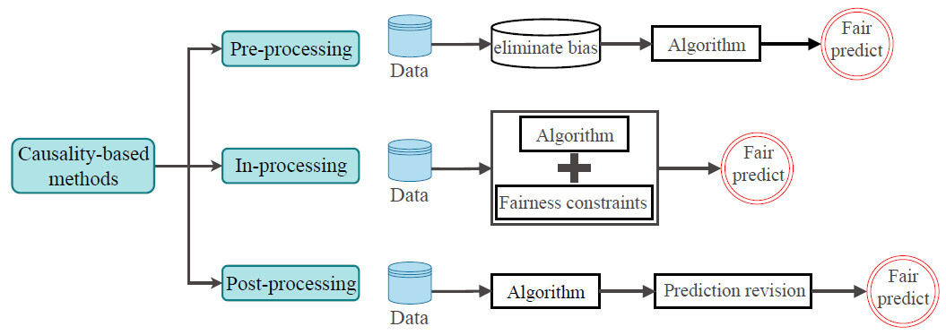
Figure 6. The categorization of causality-based fairness-enhancing approaches.
5.1. Pre-processing Causality-based methods
Pre-processing methods update the training data before feeding them into a machine learning algorithm. Specifically, one idea is to change the labels of some instances or reweigh them before training to limit the causal effects of the sensitive attributes on the decision. As a result, the classifier can make a fairer prediction [36]. On the other hand, some studies propose to reconstruct the feature representations of the data to eliminate discrimination embedded in the data [38, 39].
For example, Zhang et al.[27] formalized the presence of discrimination as the presence of a certain path-specific effect, and then framed the problem as one maximizing the likelihood subject to constraints that restrict the magnitude of the
5.2. In-Processing Causality-based methods
In-processing methods eliminate discrimination by adding constraints or regularization terms to machine learning models [46-50]. If it is allowed to change the learning procedure for a machine learning model, then in-processing can be used during the training of a model either by incorporating changes into the objective function or imposing a constraint.
For example, multi-world fairness algorithms [12] add constraints to the classification model that require satisfying the counterfactual fairness. To address the unidentifiable situation and alleviate the difficulty of determining causal models, it combines multiple possible causal models to make approximately fair predictions. A tuning parameter
5.3. Post-processing Causality-based methods
Post-processing methods modify the outcome of the decision model to make fairer decisions [55, 56]. For example, Wu et al.[57] adopted the c-component factorization to decompose the counterfactual quantity, identified the sources unidentifiable terms, and developed the lower and upper bounds of counterfactual fairness in unidentifiable situations. In the post-processing stage, they reconstructed the trained decision model so as to achieve counterfactual fairness. The counterfactual privilege algorithm [58] maximizes the overall benefit while preventing an individual from obtaining beneficial effects exceeding the threshold due to the sensitive attributes, so as to make the classifier achieve counterfactual fairness. Mishler et al.[59] suggested using doubly robust estimators to post-process a trained binary predictor in order to achieve approximate counterfactual equalized odds.
5.4. Which mechanism to use
We discuss the various mechanisms for enhancing fairness above. Here, we further compare these mechanisms and discuss the advantages and disadvantages of them, respectively. This section provides insights into how to select suitable mechanisms for use in different scenarios based on the characteristics of these mechanisms. Every type of mechanism has its advantages and disadvantages.
The pre-processing mechanism can be flexibly adapted to the downstream tasks since it can be used with any classification algorithm. However, since the pre-processing mechanism is a general mechanism where the extracted features can be widely applicable for various algorithms, there is high indeterminacy regarding the accuracy of the trained decision models.
Similar to the pre-processing mechanism, the post-processing mechanism also can be flexibly used in any decision model. Post-processing mechanisms are easier to fully eliminate discrimination for the decision models, but the accuracy of the decision models depends on the performance they obtained in the training stage [60]. Furthermore, post-processing mechanisms require access to all information of individuals during testing, which may be unavailable because of reasons of privacy protection.
The in-processing mechanism is beneficial to enable a balance between accuracy and fairness of the decision model, which is achieved by explicitly modulating the trade-off parameter in the objective function. However, such mechanisms are tightly coupled with the machine learning algorithm itself and are difficult to optimize in the application.
Based on the above discussion and the studies that attempt to comprehend which mechanism is best to use in certain situations [61, 62], we can say that there is no single mechanism that outperforms the others in all cases, and the choice of suitable mechanisms depends on the availability of sensitive variables during testing, the characteristics of the dataset, and the desired fairness measure in the application. For example, when there exists evident selection bias in a dataset, it is better to select the pre-process mechanism for use than the in-process one. Therefore, more research is needed to develop robust fairness mechanisms or to design suitable mechanisms for practical scenarios.
6. APPLICATIONS OF FAIR MACHINE LEARNING
This section enumerates different domains of machine learning and the work that has been produced by each domain to combat discrimination in their methods.
6.1. Data missing
One major challenge for fairness-enhancing algorithms is to deal with the biases inherent in the dataset that is caused by missing data. Selection biases are due to the distribution of collected data, which cannot reflect the real characteristics of disadvantaged groups. Martínez-Plumed et al.[63] learned that selection bias is mainly caused by individuals in disadvantaged groups being reluctant to disclose information, e.g., people with high incomes are more willing to share their earnings than people with low incomes, which results in bias inference that training in the training institution helps to raise earnings. To address this problem, Bareinboim et al.[64] and Spirtes et al.[65] studied how to deal with missing data and repair datasets that contain selection biases by causal reasoning, in order to improve fairness.
On the other hand, the collected data represent only one side of the reality, that is, these data do not contain any information about the population who were not selected. Biases may arise that decide which data are contained or not contained in the datasets. For example, there is a dataset that records the information of individuals whose loans were approved and the information about their ability to repay their loans. Although the automatic decision system that satisfies certain fairness requirements is constrained based on this dataset to predict whether they repay their loan on time, such a predictor may be discriminatory when it is used to assess the credit score of further applicants, since populations not approved for loans are not sufficiently representative in the training data. Goel et al.[66] used the causal graph-based framework to model the causal process of possible missing data for different settings by which different types of decisions are made in the past, and proved some data distributions can be inferred from incomplete available data based on the causal graph. Although the practical scenarios they discussed are not exhaustive, their work shows that the causal structure can be used for determining the recoverability of quantities of interest in any new scenario.
A promising solution for dealing with missing data can be found in causality-based methods. We see that causality can provide tools to improve fairness when the dataset suffers from discrimination caused by missing data.
6.2. Fair recommender Systems
Recommenders are recognized as the most effective way to alleviate information overloading. Nowadays, recommender systems have been widely used in variable applications, such as ecommerce platforms, advertisements, news articles, jobs, etc. They are not only used to analyze user behavior to infer users' preferences so as to provide them with personalized recommendations, but they also benefit content providers with more potential of making profits. Unfortunately, there exist fairness issues in recommender systems [67], which are challenging to handle and may deteriorate the effectiveness of the recommendation. The discrimination embedded in the recommender systems is mainly caused by the following aspects. User behaviors in terms of the exposed items make the observational data confounded by the exposure mechanism of recommenders and the preference of the users. Another major cause of discrimination in recommender systems is that disadvantage items reflected in the observational data are not representative. That is to say, some items may be more popular than others and thus receive more user behavior. As a result, recommender systems tend to expose users to these popular items, which results in discrimination towards unpopular items and leads to the systems not providing sufficient opportunities for minority items. Finally, one characteristic of recommender systems is the feedback loop. That is, the systems exposes to the user for determining the user behavior, which is circled back as the training data for the recommender systems. Such a feedback loop not only creates biases but also intensifies biases over time, resulting in "the rich get richer" Matthew effect.
Due to the usefulness of causal modeling [10], removing discrimination for recommender systems from a causal perspective has attracted increasing attention, where the cause graph is used for exposing potentially causal relationships from data. On the one hand, most discrimination can be understood with additional confounding factors in the causal graph and the effect of discrimination can also be inferred through the causal graph. On the other hand, recommendation can be considered as an intervention, which is similar to treating a patient with a specific drug, requiring counterfactual reasoning. What happens when recommending certain items to the users? The causal model has the potential to answer this question. For example, Wu et al.[68] focused on fairness-aware ranking and proposed to use path-specific effects to detect and remove the direct and indirect rank discrimination. Zhao et al.[69] and Zheng et al.[70] considered the effect of item popularity on user behavior and intervened in the item popularity to make fair recommendations. Zhang et al.[71] attributed popularity bias in the recommender systems to the undesirable causal effect of item popularity on items exposure and suggested intervening in the distribution of the exposed items to eliminate this causal effect. Wang et al.[72] leveraged counterfactual reasoning to eliminate the causal effect of exposure features on the prediction. Li et al.[73] proposed generating embedding vectors independent of sensitive attributes by adversarial learning to achieve counterfactual fairness. Huang et al.[74] regarded causal inference as bandits and performed
Nowadays, the explainability of recommender systems is increasingly important, which improves the persuasiveness and trustworthiness of recommendations. When addressing the fairness issues of recommender systems from the causal perspective, the explanation of recommendations can also be provided from the effects transmitted along the causal paths. Thus, we are confident that causal modeling will bring the recommendation research into a new frontier.
6.3. Fair natural language processing
Natural language processing (NLP) is an important technology for machines to understand and interpret human natural language text and realize human–computer interaction. With the development and evolution of human natural language, the natural language is characterized by a certain degree of gender, ethnicity, region, and culture. These characteristics are sensitive in certain situations, and inappropriate use can lead to prejudice and discrimination. For example, Zhao et al.[75] found that the datasets associated with multi-label object classification and visual semantic role labeling exhibit discrimination towards gender attribute, and, unfortunately, the model trained with these data would further amplify the disparity. Stanovsky et al.[76] provided multilingual quantitative evidence of gender bias in large-scale translation. They found that, among the eight target languages, all four business systems and two academic translation systems tend to translate according to stereotype rather than context. Huang et al.[77] used counterfactual evaluations to investigate whether and how language models are affected by sensitive attributes (e.g., country, occupation, and gender) to generate sentiment bias. Specifically, they used individual fairness metrics and group fairness metrics to measure counterfactual sentiment bias, conducted model training on news articles and Wikipedia corpus, and showcased the existence of sentiment bias.
Fair NLP is a kind of NLP without bias or discrimination with sensitive attributes. Shin et al.[78] proposed a counterfactual reasoning method for eliminating the gender bias of word embedding, which aims to disentangle a latent space of a given word embedding into two disjoint encoded latent spaces, namely the gender latent space and the semantic latent space, to achieve disentanglement of semantic and gender implicit descriptions. To this end, they used a gradient reversal layer to prohibit the inference about the gender latent information from semantic information. Then, they generated a counterfactual word embedding by converting the encoded gender into the opposite gender and used it to produce a gender-neutralized word embedding after geometric alignment regularization. As such, the word embedding generated by this method can strike a balance between gender debiasing and semantic information preserving. Yang and Feng [79] presented a causality-based post-processing approach for eliminating the gender bias in word embeddings. Specifically, their method was based on statistical correlation and half-sibling regression, which leverages the statistical dependency between gender-biased word vectors and gender-definition word vectors to learn the counterfactual gender information of an individual through causal inference. The learned spurious gender information is then subtracted from the gender-biased word vectors to remove the gender bias. Lu et al.[80] proposed a method called CDA to eliminate gender bias through counterfactual data augmentation. The main idea of CDA is to augment the corpus by exchanging gender word pairs in the corpus and constructing matching gender word pairs with causal interventions. As such, CDA breaks associations between gendered and gender-neutral words and alleviates the problem that gender bias increases as loss decreases when training with gradient descent.
There exists a certain degree of bias and fairness issues in word embedding, machine translation, sentiment analysis, language models, and dialog generation in NLP. At present, most studies only focus on a single bias (such as gender bias), and there is a lack of research results on other biases or eliminating multiple biases at the same time. Therefore, how should we analyze and evaluate the mechanism and impact of multi-bias in word embedding and machine learning algorithms? Establishing effective techniques for eliminating various biases in word embedding and machine learning algorithms requires further research which needs to be carried out for fair NLP.
6.4. Fair medical
Electronic health records (EHRe) contain large amounts of clinical information about heterogeneous patients and their responses to treatments. It is possible for machine learning techniques to efficiently leverage the full extent of EHRs to help physicians make predictions for patients, thus greatly improving the quality of care and reducing costs. However, because of discrimination implicitly embedded in EHRs, the automated systems may introduce or even aggravate the nursing gap between underrepresented groups and disadvantaged ones. The prior works on eliminating discrimination for clinical predictive models mostly focus on statistics-based fairness-enhancing approaches [81, 82]. In addition, they do not provide an effective evaluation of fairness to individuals, and the fairness metrics they used are difficult to verify. Some recent studies focus on assessing fairness for clinical predictive models from a causal perspective [83, 84]. For example, Pfohl et al.[83] proposed a counterfactual fairness notion to extend fairness to the individual level and leveraged variational autoencoder technology to eliminate discrimination against certain patients.
6.5. Causal analysis packages
This section introduces some representative packages or software for causal analysis, which are helpful for us to develop causality-based fairness-enhancing approaches. These packages can be roughly divided into two categories: one for discovering potential causal structure in data and the other for making causal inferences. Table 2 summarizes typical packages or software for causal analysis.
Typical packages or software for causal analysis
| Type | Package name | Program language | Description |
| Causal discovery | TETRAD [85] | Java | TETRAD is a full-featured software for causal analysis; after considerable development, it can be used to discover the causal structure behind the dataset, estimate the causal effects, simulate the causal models, etc |
| Py-causal [87] | Python | Py-causal is a Python encapsulation of TETRAD, which can call the algorithms and related functions in TETRAD | |
| Causal-learn [86] | Python | Causal-learn is the Python version of TETRAD. It provides the implementation of the latest causal discovery methods ranging from constraint-based, score-based, and constrained functional causal models-based to permutation-based methods | |
| Tigramite [88] | Python | Tigramite focuses on searching causal structure from observational time series data. | |
| gCastle [89] | Python | gCastle provides many gradient-based causal discovery approaches, as well as classic causal discovery algorithms | |
| Causal effect and Inference | CausalML [90] | Python | CausalML encapsulates many causal learning and inference approaches. One highlight of this software package is uplift modeling, which is used to evaluate the conditional average treatment effect (CATE) |
| Causaleffect [92] | R | Causaleffect is the implementation of ID algorithm | |
| DoWhy [93] | Python | DoWhy takes causal graphs as prior knowledge and uses Pearl's do-calculus method to assess causal effects | |
| Mediation [91] | R | Mediation provides model-based method and design-based method to evaluate the potential causal mechanisms. It also provides approaches to deal with common problems in practice and random trials, that is, to handle multiple mediators and evaluate causal mechanisms in case of intervention non-compliance |
TETRAD [85] is a full-featured software for causal analysis after considerable development where it can be used to discover the causal structure behind the dataset, estimate the causal effects, simulate the causal models, etc. TETRAD can accept different types of data as input, e.g., discrete data, continuous data, time series data, etc. The users can choose the appropriate well-tested causal discovery algorithms it integrates to search causal structure, as well as input prior causal knowledge to limit the search. In addition, TETRAD can parameterize the causal model and simulate the data according to the existing causal diagram. Causal-learn package [86] is the Python version of TETRAD. It provides the implementation of the latest causal discovery methods ranging from constraint-based methods, score-based methods, and constrained functional causal models-based methods to permutation-based methods. In addition, there are many packages for causal discovery [87-89]. Tigramite [88] focuses on searching causal structure from observational time series data. In addition to providing classic causal discovery algorithms, gCastle [89] provides many gradient-based causal discovery approaches.
CausalML [90] is a Python package which encapsulates many causal learning and causal inference approaches. One highlight of this package is uplift modeling, which is used to evaluate the conditional average treatment effect (CATE), that is, to estimate the impact of a treatment on a specific individual's behavior.
Mediation [91] is an R package which is used in causal mediation analysis. In other words, it provides model-based methods and design-based methods to evaluate the potential causal mechanisms. It also provides approaches to deal with common problems in practice and random trials, that is, to handle multiple mediators and evaluate causal mechanisms in case of intervention non-compliance.
Causaleffect [92] is an R package which is the implementation of ID algorithm. ID algorithm is a complete identification of causal effects algorithm, which outputs the expression of causal effect when the causal effect is identifiable or fails to run when the causal effect is unidentifiable. DoWhy [93], a Python package, also focuses on causal inference, that is, it takes causal graphs as prior knowledge and uses Pearl's
These packages used for causal analysis assist in developing causality-based fairness-enhancing methods, which are mainly reflected in exposing the causal relationship between variables and evaluating the causal effects of sensitive attributes on decision-making. However, they cannot be used directly to detect or eliminate discrimination. Although there are many software packages for detecting and eliminating discrimination, e.g., AI Fairness 360 Open Source Toolkit [94], Microsoft Research Fairlearn [95], etc, we are still lacking a package that integrates causality-based approaches.
7. CHALLENGES
Decision based on machine learning has gradually penetrated into all aspects of human society, and the fairness of its decision-making directly affects the daily life of individuals or groups, as well as users' trust and acceptance of machine learning application deployment. Recently, fair machine learning has received extensive attention, and researchers are gradually aware of the fact that relying solely on the observable data, with no additional causal information, is limited in removing discrimination, since the dataset only represents the selected population, without any information on the groups who were not selected, while such information can be achieved using knowledge of a causal graph or by a controlled experiment making use of interventions. As such, causality-based fairness machine learning algorithms have attracted more and more attention and several causality-based fairness approaches have been proposed. Although causal fairness models can indeed help us overcome many of the challenges encountered with respect to fair prediction tasks, they still face many challenges, which are discussed in the following subsections.
7.1. Causal discovery
Causality-based fairness approaches require a causal graph as additional prior knowledge of input, where the causal graph describes the mechanism by which the data are generated, that is, it reveals the causal relationship between variables. However, in practice, it is difficult for us to obtain the correct causal graph. A basic way to discover the causal relationship between variables is to conduct randomized controlled trials. Randomized controlled trials consist of randomly assigning subjects (e.g. individuals) to treatments (e.g. gender), and then comparing the outcome of all treatment groups. Unfortunately, in many cases, it may not be possible to undertake such experiments due to prohibitive costs, ethical concerns, or they are physically impossible to carry out. For example, to understand the impact of smoking, it would be necessary to force different individuals to smoke or not smoke. As another example, to understand whether hiring decision models are gender-biased, it would be necessary to change the gender of a job applicant, which is an impracticality. Researchers are therefore often left with non-experimental, observational data, and they have developed numerous methods for uncovering causal relations, i.e., causal discovery. Causal discovery algorithms can be roughly classified into the following three categories: constraint-based, score-based, and those exploiting structural asymmetries.
Constraint-based approaches conduct numerous conditional independence tests to learn about the structure of the underlying causal graph that reflects these conditional independence. Constraint-based approaches have the advantage that they are generally applicable, but the disadvantages are that faithfulness is a strong assumption and that it may require very large sample sizes to get good conditional independence tests. Furthermore, the solution of this approach to causal discovery is usually not unique, and, in particular, it does not help determine the causal direction in the two-variable case, where no conditional independence relationship is available.
Score-based algorithms use the fact that each directed acyclic graph (DAG) can be scored in relation to the data, typically using a penalized likelihood score function. The algorithms then search for the DAG that yields the optimal score. Typical scoring functions include the Bayesian information criterion [96], Bayesian–Gaussian equivalent score [96], and minimum description length (as an approximation of Kolmogorov complexity) [97, 98].
Structural asymmetry-based algorithms take into account the setting that it is impossible to infer the causal direction from observations alone when the data distribution admits structural causal models indicating either of the structural directions
In the absence of intervention and manipulation, observational data leave researchers facing a number of challenges: First, there may exist hidden confounders, which are sometimes termed the third variable problem. Second, observational data may exhibit selection bias. For example, younger patients may generally prefer surgery, while older patients may prefer medication. Third, most causal discovery algorithms are based on strong but often untestable assumptions, and applying these strong assumptions to structural or graphical models incites some harsh criticisms.
7.2. Identifiable issue
The identifiable issue is another main obstacle to the application of causal models in fair machine learning. The identifiability of causal effects, including total effect, path-specific effect, and counterfactual effect, has been extensively studied [10, 100-103]. Many causality-based fairness methods have been proposed to solve this problem so as to achieve fairness more effectively. This section summarizes the main identifiability conditions, the causality-based fairness methods that try to overcome the unidentifiable situations, and their limitations.
7.2.1. Identifiability
This review starts with the simplest identifiability condition of total effects, where the causal effect of a sensitive attribute
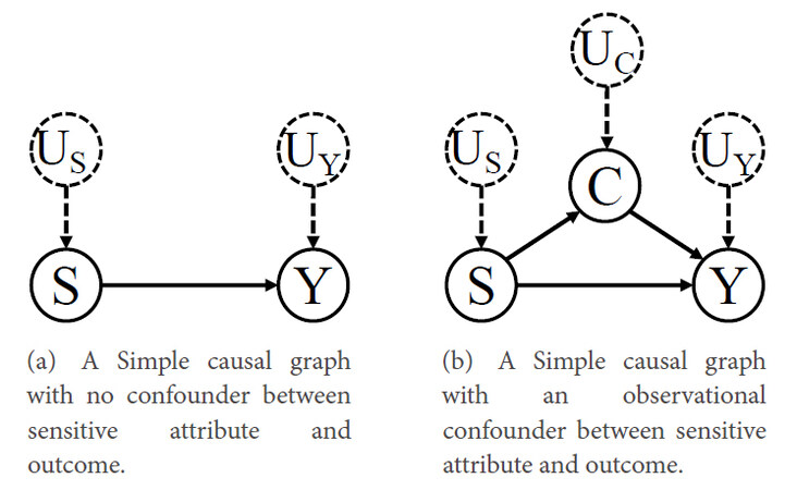
Figure 7. Simple causal graphs under Markovian assumption.
If there exists an observational confounder between
where the formula
where
For semi-Markovian models, the causal effect
where
A complex case where the causal effect of
where
Tian et al.[105] also found that, although
Moreover, the causal effect of sensitive attribute
These criteria can be generalized to the case where there is no bi-directed edges connection between the sensitive attribute and its direct children. Given the fact that the observational distribution
Shpitser et al.[15] designed a sound and complete algorithm called ID to identify all identifiable causal effects where ID outputs the expression of the causal effect for the identifiable cases. In addition, they proved that all cases of unidentifiable causal effects
As to the identifiability of counterfactual effect, if complete knowledge of the causal model is known (including structural functions,
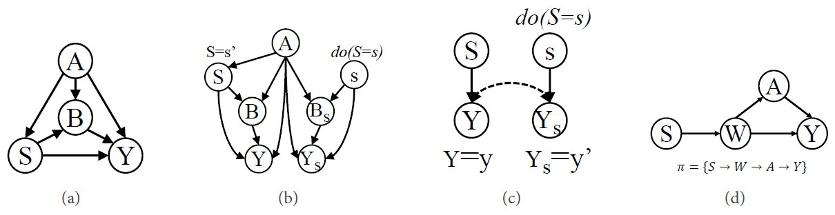
Figure 8. (a) The tony causal graph; (b) the counterfactual graph of (a); (c) the W-graph; and (d) the "kite" graph.
The analysis of the identifiability of counterfactual effect
For the identifiability of path-specific effect
7.2.2. Efforts for dealing with identifiable issues
In Section 7.2.1, we show that the causal effects are not always identifiable only from observational data and causal graphs. Several causality-based fairness methods have been proposed from different perspectives to deal with identifiable issues.
Most previous approaches tend to make simplified or even unrealistic assumptions to avoid unidentifiable situations. For example, to avoid the unidentifiable issue of the counterfactual effect, Kusner et al.[11] adopted three different assumptions: (ⅰ) only using non-descendants of the sensitive attributes to build the classifier; (ⅱ) postulating and inferring the non-deterministic sub-situations of the hidden variables based on domain knowledge; and (ⅲ) postulating the complete causal model, treating it as the additive noise model, and then estimating the errors. Zhang et al.[26] evaded the unidentifiable issue of path-specific effect caused by satisfying recanting witness criterion via changing the causal model, i.e., cutting off all causal paths from sensitive variables to the decision that pass through the redline variables. However, such simplified assumptions modify the causal model equivalent to "redefining success". Although these methods made simplified assumptions to avoid identifiable issues, such assumptions may severely damage the performance of the decision model and impose uncertainty on these methods. Besides, such simplified assumptions may modify the causal model equivalent to "redefining success", while any kind of repair is not expected within a modified model, which results in fair inferences in the real world.
Recently, some workarounds for dealing with unidentifiable situations aim to stay within the true causal model, but they obtain the true unidentifiable causal effects by developing the upper and lower bounds of the causal effects. For example, Wu et al.[57] mathematically developed the upper and lower bounds of counterfactual fairness in unidentifiable situations and used a post-processing method for reconstructing trained classifiers to make counterfactual fairness. Zhang et al.[27] mathematically bound indirect discrimination as the path-specific effect in unidentifiable cases and proposed a pre-processing method for reconstructing the observational data to remove the discrimination from the original dataset. Hu et al.[108] adopted implicit generative models and adversarial learning to estimate the upper and lower bound of average causal effect under unidentifiable cases.
One of the major reasons causal effects are not identifiable is the presence of hidden confounding. Most previous works [12, 27, 44, 57] adopt the no hidden confounders assumption (i.e., Markovian model) to facilitate the assessment of the causal effects. However, in practical scenarios, the existence of hidden confounders is an inescapable fact, since measuring all possible confounders is impossible. For example, in many cases, we cannot measure variables such as personal preferences, most genetic factors, and environmental factors. In these cases, to deal with hidden confounders and identifiable issues, many studies adopt the potential outcome framework [33, 34] and are devoted to finding so-called "proxy variables" that reflect the information of hidden confounders. For example, we cannot directly measure the socioeconomic status of patients, but patients' demographic attributes, such as their zip code, consumption ability, or employment status, can be the proxies for socioeconomic status. Variational autoencoder has been widely used to learn causal models with hidden confounders, especially for approximately inferring the complex relation between the observational variables and hidden confounders [109]. It is a computationally efficient algorithm for learning the joint distribution of the hidden confounders and the observed ones from observational data. An alternative way to eliminate the confounding bias in causal inference is to utilize the underlying network information that is attached to observational data (e.g., social networks) to infer the hidden confounders. For example, Guo et al.[110] proposed the network deconfounder to infer the influence of hidden confounders by mapping the features of observational data and auxiliary network information into the hidden space. Guo et al.[111] leveraged the network information to recognize the representation of hidden confounders. Veitch et al.[112] remarked that merely partial information that hidden confounders contain affects both the treatment and the outcome. That is to say, only a portion of confounders is actually used by the estimator to estimate the causal effects. Therefore, if a good predictive model for the treatment can be built, then one may only need to plug the outputs into a causal effect estimate directly, without any need to learn all the true confounders. Since experimental data do not suffer from hidden confounders, another method is to combine experimental and observational data together. For example, Kallus et al.[113] used limited experimental data to correct the hidden confounders in causal effect models trained on larger observational data, even if the observational data do not fully overlap with the experimental ones, which makes strictly weaker assumptions than existing approaches.
Overall, these potential outcome framework-based methods mostly rely on proxy variables. Before selecting proxy variables for hidden confounders, we need a thorough understanding of what a hidden confounder is supposed to represent, and whether there is any proxy variable that actually represents it. However, a sufficiently clear understanding may be impossible to attain in some cases.
7.3. Comprehensive definition of fairness
The sources of unfairness in machine learning algorithms are diverse and complex, and different biases have different degrees of impact on unfairness. Since most fairness notions, including causality-based fairness notions, quantify fairness in a single dimension, when comparing the capabilities of different fairness machine learning algorithms, using different fairness measures will often lead to different results. This means that, whether the algorithm is fair or not is relative, which depends not only on the model and data but also on the task requirements. There is a lack of complete and multi-dimensional causality-based fairness definition and evaluation system for fairness, and it is not possible to effectively quantify the fairness risk faced by machine learning algorithms. Therefore, we need to further explore comprehensive causal-based fairness notions and establish a comprehensive multi-dimensional evaluation system for the fairness of machine learning algorithms. In addition, the definition of fairness needs to be combined with the laws and the concept of social fairness of various countries to avoid narrow technical solutions. The proposition of PC-fairness and causality-based fairness notion defined from both macro-level and individual-level [114] are useful explorations to solve this problem.
7.4. Achieving fairness in a dynamic environment
The existing works mainly focus on studying the fairness in machine learning in static, no feedback, short-term impact scenarios, without examining how these decisions affect fairness in future applications over time and failing to effectively adapt to evolutionary cycles. At present, the research on the fairness of machine learning shows a trend of dynamic evolution, which requires the definition of fairness and algorithms to consider the dynamic, feedback, and long-term consequences of decision-making systems. This is particularly evident in recommendation systems, loans, hiring, etc. Fortunately, some researchers are modeling the long-term dynamics of fairness in these areas [115-119]. D'Amour et al.[120] regarded dynamic long-term fair learning as a Markov decision process (MDP) and proposed simulation studies to model fairness-enhancing learning in a dynamic environment. They emphasized the importance of interaction between the decision system and the environment. A complementary work [121] shows the importance of causal modeling in dynamic systems. However, due to the complexity of the real-world environment, it is impossible to model the real environment at a high level. Besides, current studies are carried out on low-dimensional data. Therefore, how to highlight important dynamics in simulations and effectively use collected data to ensure an appropriate balance between results and real-world applicability and how to adapt to high-dimensional data are current challenges. In addition, future causality-based fairness-enhancing studies can be combined with dynamic game theory for improving fairness in the confrontation environment and research the detection mechanism of dynamic fairness.
7.5. Other challenges
AI has become more and more mature after rapid development. Although most of the research on AI thus far has focused on weak AI, the design of strong AI (or human-level AI) will be increasingly vital and receive more and more attention in the near future. Weak AI only focuses on solving the given tasks input into the program, while strong AI or human-level AI (HLAI) means that its ability of thinking and action is comparable to that of a human. Therefore, developing HLAI will face more challenges. Saghiri et al.[122] comprehensively summarized the challenges of designing HLAI. As they said, unfairness issues are closely related to other challenges in AI. There is still a gap between solving the unfairness problem in AI alone and building a trustworthy AI. Next, this review discusses the relationship between fairness and the other challenges in AI.
Fairness and robustness. The robustness of the AI model is manifested in its outer generalization ability, that is, when the input data change abnormally, the performance of the AI model remains stable. AI models with poor robustness are prone to crash and, thus, fail to achieve fairness. In addition, the attacker may obtain private information about the training data and even the training data themselves, although the attacker has no illegal access to the data. However, the research on robustness is still in its infancy, and the theory and notions of robustness are still lacking currently.
Fairness and interpretability. The explainability of discrimination is very important to improving users' understanding and trust in AI models, which is even required by law in many fields. On the other hand, interpretability can explain and judge whether the fairness of AI models is satisfied or not, which assists in improving the fairness of AI models. In some important areas, e.g., healthcare, this challenge becomes more serious because it requires that any type of decision-making must be fair and interpretable.
Causality-based methods are promising solutions to these challenges, as they can not only reveal the mechanisms by which data are generated but also enable a better understanding of the causes of discrimination. Of course, there are far more challenges faced by HLAI than those above, and more about the challenges of designing HLAI can be found in Saghiri et al.'s work [122].
7.6. Future trends
More realistic application scenarios. Most of the early studies are carried out under some strong assumptions, e.g., the assumption that there are no hidden confounders between observational variables. However, these assumptions are difficult to satisfy in practical applications, which leads to erroneous evaluation. Therefore, the trained model cannot guarantee that it satisfies the fairness requirement. The current studies tend to relax these assumptions and address the unfairness issue of algorithms in more general scenarios.
Privacy protection. Due to legal requirements, sensitive attributes are often inaccessible in real applications. Fairness constraints require predictors to be in some way independent of the attributes of group members. Privacy preservation raises the same question: Is it possible to guarantee that even the strongest adversary cannot steal an individual's private information through inference attacks? Causal modeling of the problem not only is helpful to solve the fairness issue but also enables stronger privacy-preserving than statistics-based methods [123]. Combining the existing fairness mechanism with differential privacy is a promising research direction in the near future.
Build a more complete ecosystem. There is an interaction of fairness between applications in the real world. For example, in bank loans, there exists discrimination in loan quotas for groups of different genders, and this unfairness may be caused by the salary level of groups of different genders in the workplace. Therefore, we need to further explore achieving cross-domain, cross-institution collaborative fairness algorithms.
8. CONCLUSION
This review presents the relevant background, typical causality-based fairness notions, an inclusive overview of causality-based fairness methods, and their applications. The challenges of applying causality-based fairness notions in practical scenarios and future research trends on solving fairness problems in algorithms are also discussed.
Papers related to the topic of addressing fairness issues based on causality are mostly reviewed in this survey. The statistics and analysis of these papers are also carried out in this survey and the results are presented in Figure 9. Figure 9(a) reports the proportion of papers published in reputable journals or conferences, while Figure 9(b) shows the number of publications from 2017 to 2021. The research community has only recently focused on defining, measuring, and mitigating discrimination in algorithms from a causal perspective, gradually realizing the importance of causal modeling of the problems to address fairness issues.
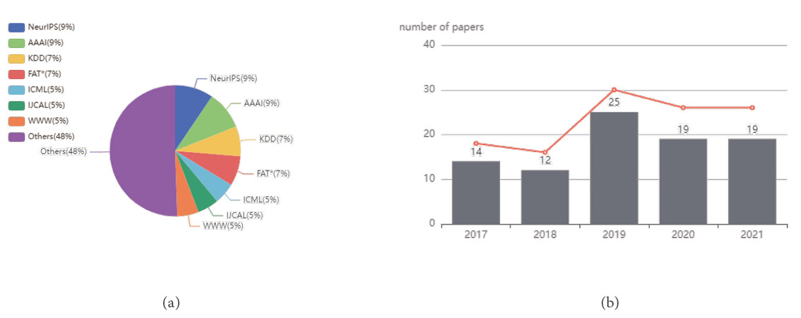
Figure 9. Statistical charts of references in this survey: (a) a pie chart that shows the proportion of publications in journals or conferences; and (b) a bar chart about the number of publications per year (from 2017 to 2021).
Therefore, we provide a relatively complete review of causality-based fairness-enhancing techniques to help researchers gain a deep understanding of this field, and we hope that more researchers will engage in this young but important field. On the one hand, discrimination detection and elimination from the causal perspective rather than statistics-based methods is more welcomed and trusted by the users of automated decision making systems, since causality-based fairness-enhancing methods consider how the data are generated and thus deeply understand the sources of discrimination. On the other hand, because of the completeness of the causal theory, it provides mathematical tools to discover discrimination when the dataset includes bias due to missing data. In addition, the main objective of this survey is to bridge the gap between the practical scenarios of discrimination elimination from the causal perspective and the ongoing theory problem. This is achieved by summing up causality-based fairness notions, approaches, and their limitations. Although the causal graph cannot be constructed without some untestable assumptions, it can still be used productively as well as serve as an auxiliary tool to incorporate scientific domain knowledge. In addition, causal graphs can exchange the causal statements that are under plausible assumptions but lack grounding in established scientific knowledge for inferring plausible conclusions. To conclude, causality-based fairness-enhancing approaches are promising solutions to reduce discrimination despite having challenges to overcome.
DECLARATIONS
Authors' contributions
Project administration: Yu G, Yan Z
Writing-original draft: Su C, Yu G, Wang J
Writing-review and editing: Yu G, Yan Z, Cui L
Availability of data and materials
Not applicable.
Financial support and sponsorship
None.
Conflicts of interest
All authors declared that they have no conflicts of interest to this work.
Ethical approval and consent to participate
Not applicable.
Consent for publication
Not applicable.
Copyright
© The Author(s) 2022.
REFERENCES
1. Cohen L, Lipton ZC, Mansour Y. Efficient candidate screening under multiple tests and implications for fairness. arXiv preprint arXiv: 190511361 2019.
2. Schumann C, Foster J, Mattei N, Dickerson J. We need fairness and explainability in algorithmic hiring. In: International Conference on Autonomous Agents and Multi-Agent Systems; 2020. pp. 1716-20.
3. Mukerjee A, Biswas R, Deb K, Mathur AP. Multi-objective evolutionary algorithms for the risk-return trade-off in bank loan management. Int Trans Operational Res 2002;9:583-97.
4. Lee MSA, Floridi L. Algorithmic fairness in mortgage lending: from absolute conditions to relational trade-offs. Minds and Machines 2021;31:165-91.
6. Berk R, Heidari H, Jabbari S, Kearns M, Roth A. Fairness in criminal justice risk assessments: The state of the art. Sociological Methods & Research 2021;50:3-44.
7. Chouldechova A. Fair prediction with disparate impact: A study of bias in recidivism prediction instruments. Big Data 2017;5:153-63.
8. Dwork C, Hardt M, Pitassi T, Reingold O, Zemel R. Fairness through awareness. In: Proceedings of the Innovations in Theoretical Computer Science Conference; 2012. pp. 214-26.
9. Hardt M, Price E, Srebro N. Equality of opportunity in supervised learning. In: Advances in Neural Information Processing Systems; 2016. pp. 3315-23.
10. Pearl J. Causality: models, reasoning and inference New York, NY, USA: Cambridge University Press; 2009.
11. Kusner MJ, Loftus J, Russell C, Silva R. Counterfactual fairness. In: Advances in Neural Information Processing Systems; 2017. pp. 4069-79.
12. Russell C, Kusner MJ, Loftus J, Silva R. When worlds collide: integrating different counterfactual assumptions in fairness. In: Advances in Neural Information Processing Systems; 2017. pp. 6414-23.
13. Pan W, Cui S, Bian J, Zhang C, Wang F. Explaining algorithmic fairness through fairness-aware causal path decomposition. In: ACM SIGKDD International Conference on Knowledge Discovery and Data Mining; 2021. pp. 1287-97.
14. Grabowicz PA, Perello N, Mishra A. Marrying fairness and explainability in supervised learning. In: ACM Conference on Fairness, Accountability, and Transparency; 2022. pp. 1905-16.
15. Shpitser I, Pearl J. Complete identification methods for the causal hierarchy. J Mach Learn Res 2008;9:1941-79.
16. Caton S, Haas C. Fairness in machine learning: A survey. arXiv preprint arXiv: 201004053 2020. Available from: https://arxiv.org/abs/2010.04053.
17. Du M, Yang F, Zou N, Hu X. Fairness in deep learning: a computational perspective. IEEE Intell Syst 2020;36:25-34.
18. Mehrabi N, Morstatter F, Saxena N, Lerman K, Galstyan A. A survey on bias and fairness in machine learning. ACM Comput Surv 2021;54:1-35.
20. Wan M, Zha D, Liu N, Zou N. Modeling techniques for machine learning fairness: a survey. arXiv preprint arXiv: 211103015 2021. Available from: https://arxiv.org/abs/2111.03015.
21. Makhlouf K, Zhioua S, Palamidessi C. On the applicability of machine learning fairness notions. ACM SIGKDD Explorations Newsletter 2021;23:14-23.
22. Makhlouf K, Zhioua S, Palamidessi C. Survey on causal-based machine learning fairness notions. arXiv preprint arXiv: 201009553 2020. Available from: https://arxiv.org/abs/2010.09553.
23. Wu D, Liu J. Involve Humans in Algorithmic Fairness Issue: A Systematic Review. In: International Conference on Information; 2022. pp. 161-76.
24. Zhang J, Bareinboim E. Fairness in decision-making—the causal explanation formula. In: AAAI Conference on Artificial Intelligence. vol. 32; 2018. pp. 2037-45.
26. Zhang L, Wu Y, Wu X. A causal framework for discovering and removing direct and indirect discrimination. In: International Joint Conference on Artificial Intelligence; 2017. pp. 3929-35.
27. Zhang L, Wu Y, Wu X. Causal modeling-based discrimination discovery and removal: Criteria, bounds, and algorithms. IEEE Trans Knowl Data Eng 2018;31:2035-50.
28. Kilbertus N, Rojas-Carulla M, Parascandolo G, et al. Avoiding discrimination through causal reasoning. In: Advances in Neural Information Processing Systems; 2017. pp. 656-66.
29. Zhang L, Wu Y, Wu X. Situation testing-based discrimination discovery: a causal inference approach. In: International Joint Conference on Artificial Intelligence; 2016. pp. 2718-24.
30. Huan W, Wu Y, Zhang L, Wu X. Fairness through equality of effort. In: The Web Conference; 2020. pp. 743-51.
31. Wu Y, Zhang L, Wu X, Tong H. Pc-fairness: a unified framework for measuring causality-based fairness. Advances in Neural Information Processing Systems 2019.
32. Khademi A, Lee S, Foley D, Honavar V. Fairness in algorithmic decision making: an excursion through the lens of causality. In: The Web Conference; 2019. pp. 2907-14.
33. Rubin DB. Estimating causal effects of treatments in randomized and nonrandomized studies. Journal of Educational Psychology 1974;66:688.
34. Splawa-Neyman J, Dabrowska DM, Speed T. On the application of probability theory to agricultural experiments. Essay on principles. Section 9. Statist Sci 1990:465-72.
35. Bendick M. Situation testing for employment discrimination in the United States of America. Horizons stratégiques 2007;5:17-39.
36. Luong BT, Ruggieri S, Turini F. k-NN as an implementation of situation testing for discrimination discovery and prevention. In: ACM SIGKDD International Conference on Knowledge Discovery and Data Mining; 2011. pp. 502-10.
37. Imbens GW, Rubin DB. Causal inference in statistics, social, and biomedical sciences 2015.
38. Zemel R, Wu Y, Swersky K, Pitassi T, Dwork C. Learning fair representations. In: International Conference on Machine Learning; 2013. pp. 325-33.
39. Feldman M, Friedler SA, Moeller J, Scheidegger C, Venkatasubramanian S. Certifying and removing disparate impact. In: proceedings of the ACM SIGKDD International Conference on Knowledge Discovery and Data Mining; 2015. pp. 259-68.
40. Xu D, Wu Y, Yuan S, Zhang L, Wu X. Achieving causal fairness through generative adversarial networks. In: International Joint Conference on Artificial Intelligence; 2019. pp. 1452-58.
41. Kocaoglu M, Snyder C, Dimakis AG, Vishwanath S. CausalGAN: Learning causal implicit generative models with adversarial training. In: International Conference on Learning Representations; 2018.
42. Salimi B, Howe B, Suciu D. Data management for causal algorithmic fairness. IEEE Data Eng Bull 2019: 24-35. Available from: http://sites.computer.org/debull/A19sept/p24.pdf.
43. Salimi B, Rodriguez L, Howe B, Suciu D. Interventional fairness: Causal database repair for algorithmic fairness. In: International Conference on Management of Data; 2019. pp. 793-810.
44. Nabi R, Shpitser I. Fair inference on outcomes. In: AAAI Conference on Artificial Intelligence; 2018.
45. Chiappa S. Path-specific counterfactual fairness. In: AAAI Conference on Artificial Intelligence; 2019. pp. 7801-8.
46. Agarwal A, Beygelzimer A, Dudík M, Langford J, Wallach H. A reductions approach to fair classification. In: International Conference on Machine Learning; 2018. pp. 60-69. [DOI: http://proceedings.mlr.press/v80/agarwal18a.html].
47. Bechavod Y, Ligett K. Learning fair classifiers: a regularization-inspired approach. arXiv preprint arXiv: 170700044 2017. Available from: http://arxiv.org/abs/1707.00044.
48. Kamishima T, Akaho S, Asoh H, Sakuma J. Fairness-aware classifier with prejudice remover regularizer. In: Joint European Conference on Machine Learning and Knowledge Discovery in Databases; 2012. pp. 35-50.
49. Zafar MB, Valera I, Rogriguez MG, Gummadi KP. Fairness constraints: mechanisms for fair classification. In: Artificial Intelligence and Statistics; 2017. pp. 962-70. Available from: http://proceedings.mlr.press/v54/zafar17a.html.
50. Zafar MB, Valera I, Gomez Rodriguez M, Gummadi KP. Fairness beyond disparate treatment and disparate impact: learning classification without disparate mistreatment. In: The Web Conference; 2017. pp. 1171-80.
51. Hu Y, Wu Y, Zhang L, Wu X. Fair multiple decision making through soft interventions. Adv Neu Inf Pro Syst 2020;33:17965-75.
52. Garg S, Perot V, Limtiaco N, et al. Counterfactual fairness in text classification through robustness. In: Proceedings of the AAAI/ACM Conference on AI, Ethics, and Society; 2019. pp. 219-26.
53. Di Stefano PG, Hickey JM, Vasileiou V. Counterfactual fairness: removing direct effects through regularization. arXiv preprint arXiv: 200210774 2020. Available from: https://arxiv.org/abs/2002.10774.
54. Kim H, Shin S, Jang J, et al. Counterfactual fairness with disentangled causal effect variational autoencoder. In: AAAI Conference on Artificial Intelligence; 2021. pp. 8128-36. Available from: https://ojs.aaai.org/index.php/AAAI/article/view/16990.
55. Corbett-Davies S, Pierson E, Feller A, Goel S, Huq A. Algorithmic decision making and the cost of fairness. In: Proceedings of the ACM SIGKDD International Conference on Knowledge Discovery and Data Mining; 2017. pp. 797-806.
56. Dwork C, Immorlica N, Kalai AT, Leiserson M. Decoupled classifiers for group-fair and efficient machine learning. In: International Conference on Fairness, Accountability and Transparency; 2018. pp. 119-33. http://proceedings.mlr.press/v81/dwork18a.html.
57. Wu Y, Zhang L, Wu X. Counterfactual fairness: unidentification, bound and algorithm. In: International Joint Conference on Artificial Intelligence; 2019. pp. 1438-44.
58. Kusner M, Russell C, Loftus J, Silva R. Making decisions that reduce discriminatory impacts. In: International Conference on Machine Learning; 2019. pp. 3591-600. Available from: http://proceedings.mlr.press/v97/kusner19a/kusner19a.pdf.
59. Mishler A, Kennedy EH, Chouldechova A. Fairness in risk assessment instruments: post-processing to achieve counterfactual equalized odds. In: ACM Conference on Fairness, Accountability, and Transparency; 2021. pp. 386-400.
60. Woodworth B, Gunasekar S, Ohannessian MI, Srebro N. Learning non-discriminatory predictors. In: Conference on Learning Theory; 2017. pp. 1920-53. Available from: http://proceedings.mlr.press/v65/woodworth17a.html.
61. Calders T, Verwer S. Three naive Bayes approaches for discrimination-free classification. Data Min Knowl Discov 2010;21:277-92.
62. Friedler SA, Scheidegger C, Venkatasubramanian S, et al. A comparative study of fairness-enhancing interventions in machine learning. In: Proceedings of the Conference on Fairness, Accountability, and Transparency; 2019. pp. 329-38.
63. Martínez-Plumed F, Ferri C, Nieves D, Hernández-Orallo J. Fairness and missing values. arXiv preprint arXiv: 190512728 2019. Available from: http://arxiv.org/abs/1905.12728.
64. Bareinboim E, Pearl J. Causal inference and the data-fusion problem. Proc Natl Acad Sci 2016;113:7345-52.
65. Spirtes P, Meek C, Richardson T. Causal inference in the presence of latent variables and selection bias. In: Conference on Uncertainty in Artificial Intelligence; 1995. pp. 499-506.
66. Goel N, Amayuelas A, Deshpande A, Sharma A. The importance of modeling data missingness in algorithmic fairness: a causal perspective. In: AAAI Conference on Artificial Intelligence. vol. 35; 2021. pp. 7564-73. Available from: https://ojs.aaai.org/index.php/AAAI/article/view/16926.
67. Burke R. Multisided fairness for recommendation. arXiv preprint arXiv: 170700093 2017. Available from: http://arxiv.org/abs/1707.00093.
68. Wu Y, Zhang L, Wu X. On discrimination discovery and removal in ranked data using causal graph. In: Proceedings of the ACM SIGKDD International Conference on Knowledge Discovery and Data Mining; 2018. pp. 2536-44.
69. Zhao Z, Chen J, Zhou S, et al. Popularity Bias Is Not Always Evil: Disentangling Benign and Harmful Bias for Recommendation. arXiv preprint arXiv: 210907946 2021. Available from: https://arxiv.org/abs/2109.07946.
70. Zheng Y, Gao C, Li X, et al. Disentangling user interest and conformity for recommendation with causal embedding. In: The Web Conference; 2021. pp. 2980-91.
71. Zhang Y, Feng F, He X, et al. Causal intervention for leveraging popularity bias in recommendation. In: Proceedings of the 44th International ACM SIGIR Conference on Research and Development in Information Retrieval; 2021. pp. 11-20.
72. Wang W, Feng F, He X, Zhang H, Chua TS. Clicks can be cheating: counterfactual recommendation for mitigating clickbait issue. In: Proceedings of the 44th International ACM SIGIR Conference on Research and Development in Information Retrieval; 2021. pp. 1288-97.
73. Li Y, Chen H, Xu S, Ge Y, Zhang Y. Towards personalized fairness based on causal notion. In: International ACM SIGIR Conference on Research and Development in Information Retrieval; 2021. pp. 1054-63.
74. Huang W, Zhang L, Wu X. Achieving counterfactual fairness for causal bandit. In: AAAI Conference on Artificial Intelligence; 2022. pp. 6952-59.
75. Zhao J, Wang T, Yatskar M, Ordonez V, Chang KW. Men also like shopping: reducing gender bias amplification using corpus-level constraints. In: Conference on Empirical Methods in Natural Language Processing; 2017. pp. 2979-89.
76. Stanovsky G, Smith NA, Zettlemoyer L. Evaluating gender bias in machine translation. In: Proceedings of the 57th Annual Meeting of the Association for Computational Linguistics; 2019. pp. 1679-84.
77. Huang PS, Zhang H, Jiang R, et al. Reducing sentiment bias in language models via counterfactual evaluation. arXiv preprint arXiv: 191103064 2019.
78. Shin S, Song K, Jang J, et al. Neutralizing gender bias in word embeddings with latent disentanglement and counterfactual generation. In: Empirical Methods in Natural Language Processing Conference; 2020. pp. 3126-40.
79. Yang Z, Feng J. A causal inference method for reducing gender bias in word embedding relations. In: AAAI Conference on Artificial Intelligence; 2020. pp. 9434-41.
80. Lu K, Mardziel P, Wu F, Amancharla P, Datta A. Gender bias in neural natural language processing. In: Logic, Language, and Security; 2020. pp. 189-202.
81. Chen IY, Szolovits P, Ghassemi M. Can AI help reduce disparities in general medical and mental health care? AMA J Ethics 2019;21:167-79.
83. Pfohl SR, Duan T, Ding DY, Shah NH. Counterfactual reasoning for fair clinical risk prediction. In: Machine Learning for Healthcare Conference; 2019. pp. 325-58. Available from: http://proceedings.mlr.press/v106/pfohl19a.html.
84. Pfohl SR, Foryciarz A, Shah NH. An empirical characterization of fair machine learning for clinical risk prediction. J Biomed Inform 2021;113:103621.
85. Ramsey JD, Zhang K, Glymour M, et al. TETRAD—A toolbox for causal discovery. In: International Workshop on Climate Informatics; 2018. Available from: http://www.phil.cmu.edu/tetrad/.
86. Zhang K, Ramsey J, Gong M, et al. Causal-learn: Causal discovery for Python; 2022. https://github.com/cmu-phil/causal-learn.
87. Wongchokprasitti CK, Hochheiser H, Espino J, et al. . bd2kccd/py-causal v1.2.1; 2019. https://doi.org/10.5281/zenodo.3592985.
88. Runge J, Nowack P, Kretschmer M, Flaxman S, Sejdinovic D. Detecting and quantifying causal associations in large nonlinear time series datasets. Sci Adv 2019;5:eaau4996.
89. Zhang K, Zhu S, Kalander M, et al. gCastle: a python toolbox for causal discovery. arXiv preprint arXiv: 211115155 2021. Available from: https://arxiv.org/abs/2111.15155.
90. Chen H, Harinen T, Lee JY, Yung M, Zhao Z. Causalml: Python package for causal machine learning. arXiv preprint arXiv: 200211631 2020. Available from: https://arxiv.org/abs/2002.11631.
91. Tingley D, Yamamoto T, Hirose K, Keele L, Imai K. mediation: R package for causal mediation analysis. J Stat Softw 2014;59:1-38.
92. Tikka S, Karvanen J. Identifying causal effects with the R Package causaleffect. J Stat Softw 2017;76:1-30.
93. Sharma A, Kiciman E. DoWhy: an end-to-end library for causal inference. arXiv preprint arXiv: 201104216 2020. Available from: https://arxiv.org/abs/2011.04216.
94. Bellamy RK, Dey K, Hind M, et al. AI Fairness 360: An extensible toolkit for detecting and mitigating algorithmic bias. IBM J Res Dev 2019;63:1-15.
95. Bird S, Dudík M, Edgar R, et al. Fairlearn: A toolkit for assessing and improving fairness in AI. Technical Report MSR-TR-2020-32, Microsoft 2020.
96. Geiger D, Heckerman D. Learning gaussian networks. In: Conference on Uncertainty in Artificial Intelligence; 1994. pp. 235-43.
97. Janzing D, Schölkopf B. Causal inference using the algorithmic Markov condition. IEEE Trans Inf Theory 2010;56:5168-94.
98. Kalainathan D, Goudet O, Guyon I, Lopez-Paz D, Sebag M. Structural agnostic modeling: adversarial learning of causal graphs. arXiv preprint arXiv: 180304929 2018. Available from: https://doi.org/10.48550/arXiv.1803.04929.
99. Hoyer PO, Shimizu S, Kerminen AJ, Palviainen M. Estimation of causal effects using linear non-Gaussian causal models with hidden variables. Int J Approx Reason 2008;49:362-78.
100. Huang Y, Valtorta M. Identifiability in causal Bayesian networks: a sound and complete algorithm. In: National Conference on Artificial Intelligence; 2006. pp. 1149-54.
101. Tian J. Identifying linear causal effects. In: AAAI Conference on Artificial Intelligence; 2004. pp. 104-11.
102. Shpitser I. Counterfactual graphical models for longitudinal mediation analysis with unobserved confounding. Cogn Sci 2013;37:1011-35.
103. Malinsky D, Shpitser I, Richardson T. A potential outcomes calculus for identifying conditional path-specific effects. In: International Conference on Artificial Intelligence and Statistics; 2019. pp. 3080-88. Available from: http://proceedings.mlr.press/v89/malinsky19b.html. [PMID: 31886462]31886462PMC6935349.
104. Shpitser I, Pearl J. Identification of conditional interventional distributions. In: Conference on Uncertainty in Artificial Intelligence; 2006. pp. 437-44.
105. Tian J, Pearl J. A general identification condition for causal effects. eScholarship, University of California; 2002.
106. Shpitser I, Pearl J. What counterfactuals can be tested. In: Conference on Uncertainty in Artificial Intelligence; 2007. pp. 352-59.
107. Avin C, Shpitser I, Pearl J. Identifiability of path-specific effects. In: International Joint Conference on Artificial Intelligence; 2005. pp. 357-63.
108. Hu Y, Wu Y, Zhang L, Wu X. A generative adversarial framework for bounding confounded causal effects. In: AAAI Conference on Artificial Intelligence; 2021. p. 12104–12112. Available from: https://ojs.aaai.org/index.php/AAAI/article/view/17437.
109. Louizos C, Shalit U, Mooij JM, et al. Causal effect inference with deep latent-variable models; 2017. pp. 6446-56.
110. Guo R, Li J, Liu H. Learning individual causal effects from networked observational data. In: International Conference on Web Search and Data Mining; 2020. pp. 232-40.
111. Guo R, Li J, Liu H. Counterfactual evaluation of treatment assignment functions with networked observational data. In: Proceedings of the SIAM International Conference on Data Mining; 2020. pp. 271-79.
112. Veitch V, Wang Y, Blei D. Using embeddings to correct for unobserved confounding in networks; 2019. pp. 13769-79.
113. Kallus N, Puli AM, Shalit U. Removing hidden confounding by experimental grounding; 2018. pp. 10888-97.
114. Mhasawade V, Chunara R. Causal multi-level fairness. In: Proceedings of the AAAI/ACM Conference on AI, Ethics, and Society; 2021. pp. 784-94.
116. Hu L, Chen Y. A short-term intervention for long-term fairness in the labor market. In: The Web Conference; 2018. pp. 1389-98.
117. Mouzannar H, Ohannessian MI, Srebro N. From fair decision making to social equality. In: Proceedings of the Conference on Fairness, Accountability, and Transparency; 2019. pp. 359-68.
118. Bountouridis D, Harambam J, Makhortykh M, et al. Siren: A simulation framework for understanding the effects of recommender systems in online news environments. In: Proceedings of the Conference on Fairness, Accountability, and Transparency; 2019. pp. 150-59.
119. Kannan S, Roth A, Ziani J. Downstream effects of affirmative action. In: Proceedings of the Conference on Fairness, Accountability, and Transparency; 2019. pp. 240-48.
120. D'Amour A, Srinivasan H, Atwood J, et al. Fairness is not static: deeper understanding of long term fairness via simulation studies. In: Proceedings of the Conference on Fairness, Accountability, and Transparency; 2020. pp. 525-34.
121. Creager E, Madras D, Pitassi T, Zemel R. Causal modeling for fairness in dynamical systems. In: International Conference on Machine Learning; 2020. pp. 2185-95.
122. Saghiri AM, Vahidipour SM, Jabbarpour MR, Sookhak M, Forestiero A. A Survey of Artificial Intelligence Challenges: Analyzing the Definitions, Relationships, and Evolutions. App Sci 2022;12:4054.
Cite This Article
Export citation file: BibTeX | RIS
OAE Style
Su C, Yu G, Wang J, Yan Z, Cui L. A review of causality-based fairness machine learning. Intell Robot 2022;2(3):244-74. http://dx.doi.org/10.20517/ir.2022.17
AMA Style
Su C, Yu G, Wang J, Yan Z, Cui L. A review of causality-based fairness machine learning. Intelligence & Robotics. 2022; 2(3): 244-74. http://dx.doi.org/10.20517/ir.2022.17
Chicago/Turabian Style
Su, Cong, Guoxian Yu, Jun Wang, Zhongmin Yan, Lizhen Cui. 2022. "A review of causality-based fairness machine learning" Intelligence & Robotics. 2, no.3: 244-74. http://dx.doi.org/10.20517/ir.2022.17
ACS Style
Su, C.; Yu G.; Wang J.; Yan Z.; Cui L. A review of causality-based fairness machine learning. Intell. Robot. 2022, 2, 244-74. http://dx.doi.org/10.20517/ir.2022.17
About This Article
Copyright

Data & Comments
Data


 Cite This Article 37 clicks

 Like This Article 1
likes
Like This Article 1
likes


Comments
Comments must be written in English. Spam, offensive content, impersonation, and private information will not be permitted. If any comment is reported and identified as inappropriate content by OAE staff, the comment will be removed without notice. If you have any queries or need any help, please contact us at support@oaepublish.com.