College of Electronic and Information Engineering, Tongji University, Shanghai 201804, China.
College of Transportation Engineering, Tongji University, Shanghai 201804, China.
Correspondence to: Prof. Hao Zhang, College of Electronic and Information Engineering, Tongji University, 4800, Cao'an Road, Shanghai 201804, China. E-mail: zhang_hao@tongji.edu.cn
Received: 6 Jun 2022 | First Decision: 19 Jul 2022 | Revised: 31 Jul 2022 | Accepted: 10 Aug 2022 | Published: 20 Aug 2022
This paper focuses on the leader-following consensus problem of discrete-time multi-agent systems subject to channel fading under switching topologies. First, a topology switching-based channel fading model is established to describe the information fading of the communication channel among agents, which also considers the channel fading from leader to follower and from follower to follower. It is more general than models in the existing literature that only consider follower-to-follower fading. For discrete multi-agent systems, the existing literature usually adopts time series or Markov process to characterize topology switching while ignoring the more general semi-Markov process. Based on the advantages and properties of semi-Markov processes, discrete semi-Markov jump processes are adopted to model network topology switching. Then, the semi-Markov kernel approach for handling discrete semi-Markov jumping systems is exploited and some novel sufficient conditions to ensure the leader-following mean square consensus of closed-loop systems are derived. Furthermore, the distributed consensus protocol is proposed by means of the stochastic Lyapunov stability theory so that the underlying systems can achieve ℋ∞ consensus performance index. In addition, the proposed method is extended to the scenario where the semi-Markov kernel of semi-Markov switching topologies is not completely accessible. Finally, a simulation example is given to verify the results proposed in this paper. Compared with the existing literature, the method in this paper is more effective and general.
With the rapid development of computer technology and networks, distributed cooperative control has drawn increasing attention due to its application in various fields, especially computer science and automation control. A fundamental and important research topic of distributed system control is the consensus problem of multi-agent systems. It has attracted considerable interest among many researchers in different fields in the past few decades, due to its significant applications in civilians and militaries, such as unmanned air vehicles [1-3], autonomous underwater vehicles [4], multiple surface vessels [5], robot formation [6, 7]. The consensus problem essentially refers to a team of agents reaching the same state by designing proper and available distributed control algorithms that only utilize local information exchange with neighbors. Over the past decade, there have been a wealth of interesting and instructive achievements focusing on consensus problem of multi-agent systems, including leaderless consensus [8-13] and leader-following consensus [14-21]. The leaderless output consensus problem of multi-agent systems composed of agents with different orders was studied by transforming the original system through feedback linearization. Static feedback and dynamic feedback controllers are designed to solve the consensus problem and sinusoidal synchronization problem under uniformly jointly strongly connected topologies [8]. Under cyber-attacks, literature [9] proposed a fully distributed adaptive control protocol to solve the leaderless consensus problem of uncertain high-order nonlinear systems. The work [11] discussed the event-triggered coordination problem for general linear multi-agent systems based on a Lyapunov equation method. Leader-following consensus means that the states of all follower agents are expected to approach the state of the leader agent. In many practical situations, leader-following consensus can accomplish more complex tasks by enhancing inter-agent communication. Compared with leaderless consensus, leader-following consensus can be beneficial in reducing control costs and save energy. The key to the leader-follower consensus problem is how to design a distributed control protocol to synchronize the states of all follower agents and the leader agent. The work [14] proposed a novel distributed observer-type consensus controller for high-order stochastic strict feedback multi-agent systems based only on relative output measurements of neighbors. The 1-moment exponential leader-following consensus of the underlying system is ensured by adopting appropriate state transformation. In [15], the sampled-data leader-following consensus problem for a family of general linear multi-agent systems was addressed, and the distributed asynchronous sampled-data state feedback control law was designed. The event-based secure leader-following consensus control problem of multi-agent systems with multiple cyber attacks, which contain reply attacks and DoS attacks simultaneously, was studied in [16]. The fixed-time leader-following group consensus of multi-agent systems composed of first-order integrators was realized under a directed graph[17]. By designing a nonlinear distributed controller, the follower agents of every group can reach an agreement with its corresponding leader within a specified convergence time. In [19], the author considered the problem of resilient practical cooperative output regulation of heterogeneous linear multi-agent systems, in which the dynamics of exosystem are unknown and switched under DOS attacks. A new cooperative output regulation scheme consisting of distributed controller, distributed resilient observer, auxiliary observer and data-driven learning algorithm was proposed to ensure the global uniform boundedness of the regulated output. More results can be seen in [18, 20, 21] and references cited therein.
It is well known that there is a large amount of data transmission in the control process of multi-agents. Data packets or signals between agents are usually transmitted through wireless communication networks. However, some special physical phenomena (such as reflection, refraction, diffraction) may occur during the transmission of a signal or data packet through a communication link or channel, which will result in the loss of signal energy and lead to the signal distorted. This type of phenomenon is often referred to the channel fading. Typically, fading effects are closely related to multipath propagation and shadows from obstacles. In practical applications, the factors that cause channel fading mainly include time, geographic location, and radar frequency. As a result, the phenomenon of channel fading may result in the degradation of signal quality due to the inability to receive accurate transmission information, thereby deteriorating the desired performance of the system. This also shows that it is meaningful to consider channel fading effects for the distributed control of multi-agent systems. In view of this, some results on channel fading have been published, such as channel fading of single systems [22-26], channel fading for multi-agent systems [27-29]. The reference [22] designed a nonparallel distribution compensation interval type-2 fuzzy controller to address dynamic event-triggered control problems for interval type-2 fuzzy systems subject to fading channel, where the fading phenomenon is characterized by a time-varying random process. The literature [23] focused on the finite-horizon $$ H_{\infty} $$ state estimation problem of periodic neural networks subject to multi-fading channels. By employing the stochastic analysis method and introducing a set of correlated random variables, sufficient criteria to ensure the stochastic stability of the estimation error system with correlated fading channels were obtained and the desired $$ H_{\infty} $$ performance was achieved. In [25], the event-triggered asynchronous guaranteed that cost control problem for Markov jump neural networks subject to fading channels could be addressed, where a novel rice fading model was established to consider the effects of signal reflections and shadows in wireless networks. The consensus tracking problem of second-order multi-agent systems with channel fading was investigated using the sliding mode control method, and the feasible distributed sliding mode controller was designed by introducing the statistical information of channel fading to the measure functions of the consensus errors [27]. It should be pointed out that most of the literatures mentioned above on channel fading in multi-agent systems only consider the fading effect among the follower agents and ignore the fading effect between the leader agent and the follower agents. As stated earlier, the leader plays a crucial role in the leader-following consensus problem. To improve the applicability of the controller and the ability to deal with the problem, it is reasonable and necessary to consider both the fading effect of leader-to-follower and follower-to-follower agents at the same time in the channel fading problem of multi-agent systems. This is one of the motivations of this paper.
On the other hand, the communication topology of multi-agent systems may change in practice due to various factors, such as sudden changes in the environment, communication range limitations, link failures, packet loss, malicious cyber attacks, etc. Given this, many researchers assume that the topology among agents is time-varying or Markov switching. Some good consensus results for multi-agent systems under time-varying topology and Markov switching topology have been reported in the past decade [30-34]. For example, the work [33] investigated the coupled group consensus problem for general linear time-invariant multi-agent systems under continuous-time homogeneous Markov switching topology. The designed linear consensus protocol can achieve coupled group consensus of the considered system under some algebraic and topological conditions. It is worth noting that since the transition probability in Markov jump process is constant and there is no memory characteristic, there are still some limitations in using Markov jump process to model topology switching among agents. Recently, a class of more general semi-Markov jump processes with a non-exponential distribution of sojourn-time (the time interval between two consecutive jumps) and time-varying transition probabilities has attracted interest of many scholars and has been used to characterize the topological switching among agents [35-38]. For example, the leader-following consensus of a multi-agent system under a sampled-data-based event-triggered transmission scheme was realized [35], where a semi-Markov jump process was employed to model the switching of the network topologies. The containment control problem concerning semi-Markov jump multi-agent systems with semi-Markov switching topologies was studied by designing static and dynamic containment controllers [37]. Under a semi-Markov switching topology with partially unknown transition rates, the $$ H_{\infty} $$ leader-follower consensus control of a class of nonlinear multi-agent systems with external perturbations was achieved, and sufficient conditions for ensuring system consistency and $$ H_{\infty} $$ performance were derived based on the linear matrix inequality form [38]. However, most of the above literature on semi-Markov switching topology is considered for the continuous system case. As a matter of fact, in the discrete-time case, the semi-Markov jump process can exert a stronger modeling ability and have a larger application range. The reason is that the probability density function of sojourn-time in the discrete semi-Markov jump process can be of different types in different modes, or of the same type but with different parameters. In order to make the modeling of switching topology more realistic, it is very necessary and valuable to employ discrete-time semi-Markov switching topologies. Naturally, how to deal with the consensus problem of multi-agent systems in this situation is a key point. Recently, the discrete semi-Markov jump process was adopted to model general linear systems and a semi-Markov kernel method was proposed to address its stability and stabilization problems [39, 40]. This also provides an idea for solving the consensus problem of multi-agent systems under discrete semi-Markov switching topology. To the best of our knowledge, to date, there have been few results on the leader-following consensus problem for discrete-time multi-agent systems subject to channel fading under semi-Markov switching topologies. Therefore, how to design a suitable distributed control protocol and how to establish leader-following consensus criteria for multi-agent systems with channel fading under discrete semi-Markov switching topologies are the key issues. This inspires us to carry out this work.
Motivated by the above discussion, in this paper, the $$ \mathcal{H}_{\infty} $$ leader-following consensus problem of discrete multi-agent systems with channel fading is investigated under the premise of semi-Markov switching topology. The major contributions of this paper can be highlighted as follows: (Ⅰ) Compared with the literature [27, 41], a more general channel fading model based on discrete semi-Markov switching topologies is established to characterize the possible effects of inter-agent signal transmission. The influences of channel fading between leader and follower, follower and follower agents are simultaneously considered to explore the influence of channel fading on system consensus, rather than considering only channel fading among follower agents in literature [27, 41]. (Ⅱ) As mentioned in the previous paragraph, discrete semi-Markov processes are more powerful in modeling ability and application range than Markov and continuous-time semi-Markov processes. For this reason, different from the Markov switching and continuous-time semi-Markov switching topologies adopted in [32-38], this paper employs a discrete semi-Markov process to describe the network topology switching among agents and switching for channel fading. A set of novel sufficient conditions to guarantee that leader-following mean square consensus of multi-agent systems under semi-Markov switching topologies is derived via a semi-Markov kernel approach. (Ⅲ) The distributed consensus controller design scheme based on fading relative states is proposed to solve the $$ \mathcal{H}_{\infty} $$ leader-following consensus control problem when the semi-Markov kernel of switching topologies is fully accessible and incompletely accessible, respectively. The rest of this paper is organized as follows. The preliminaries and problem formulation are given in section Ⅱ. Section Ⅲ presents the main results. Then, simulation examples are provided in Section Ⅳ. Finally, the conclusion and future work are introduced in Section Ⅴ.
Notations: Denote that $$ \mathbb{R}^{n} $$ and $$ \mathbb{R}^{n\times n} $$ be the sets of $$ n $$-dimensional vectors and $$ n\times n $$ real matrices. $$ \mathbb{N} $$ represents the sets of nonnegative integers. The sets of positive integers is denoted by $$ \mathbb{N}^{+} $$. $$ \mathbb{N}_{\geq b_{1}} $$ and $$ \mathbb{N}_{[b_{1},b_{2}]} $$ stand for the sets $$ \{c\in\mathbb{N}|b\geq b_{1}\} $$ and $$ \{b\in\mathbb{N}|b_{1}\leq b\leq b_{2}\} $$, respectively. A matrix $$ Q\succ 0 (\prec 0) $$ indicates it is positive (negative) definite. A $$ N\times N $$ identity matrix is defined as $$ I_{N} $$. Denote a symmetric term in a matrix by $$ * $$. $$ \otimes $$ refers to the Kronecker product. Moreover, $$ \mathbb{E}\{\cdot\} $$ and $$ \|x\| $$ represent the mathematical expectation operator and the Euclidean norm of the vectors. If not specifically stated, matrices and vectors have appropriate dimensions.
2. PRELIMINARIES AND PROBLEM FORMULATION
2.1. Graph theory
In this paper, we employed an undirected graph $$ \mathcal{G}=\{\mathcal{V},\mathcal{E},\mathcal{A}\} $$ to depict the information interaction topology among $$ N $$ agents. $$ \mathcal{V}=\{v_{1},v_{2},...,v_{N}\} $$ stands for the node sets, in which $$ v_{i} $$ is the $$ i $$th agent. $$ \mathcal{E}\subset\mathcal{V}\times\mathcal{V} $$ represents a set of edges. The adjacency matrix associated with graph $$ \mathcal{G} $$ is denoted by $$ \mathcal{A}=[a_{ij}]\in \mathbb{R}^{N\times N} $$. If node $$ v_{i} $$ can receive information from node $$ v_{j} $$, there is an edge $$ (v_{j},v_{i}) $$ between node $$ v_{i} $$ and node $$ v_{j} $$. The elements $$ a_{ij} $$ of matrix $$ \mathcal{A} $$ is weighted coefficient of edge $$ (v_{j},v_{i}) $$, and $$ a_{ij}>0 $$, if $$ (v_{j},v_{i})\in \mathcal{E} $$, otherwise, $$ a_{ij}=0 $$. Self-loop is not considered. The set of neighbors of node $$ v_{i} $$ can be represented as $$ \mathcal{N}_{i}=\{v_{j}\in \mathcal{V}|(v_{j},v_{i})\in \mathcal{E}\} $$. The degree matrix of graph $$ \mathcal{G} $$ is denoted as $$ \mathcal{D}=diag\{d_{i}\}\in \mathbb{R}^{N\times N} $$, where $$ d_{i}=\sum_{j\in \mathcal{N}_{i}}a_{ij} $$. Then, one can obtain that the Laplacian matrix is $$ \mathcal{L}=\mathcal{D}-\mathcal{A} $$. Denote matrix $$ \mathcal{M}=diag\{m_{i}\}\in \mathbb{R}^{N\times N} $$, where $$ m_{i} $$ stands for the information exchange of node $$ v_{i} $$ and leader node. If node $$ v_{i} $$ can access the information of the leader, $$ m_{i}=1 $$, otherwise, $$ m_{i}=0 $$.
2.2. Problem formulation
Consider a linear discrete-time multi-agent system consist of one leader and $$ N $$ follower agents:
where $$ x_{i}(k)\in\mathbb{R}^{n_{x}} $$, $$ u_{i}(k)\in\mathbb{R}^{m} $$, $$ x_{0}(k)\in\mathbb{R}^{n_{x}} $$ are the state, input of the $$ i $$th follower, the state of leader, respectively. Matrices $$ A\in\mathbb{R}^{n_{x}\times n_{x}} $$ and $$ B\in\mathbb{R}^{n_{x}\times m} $$ represent known constant system matrices.
In the real world, the communication network topology among agents is more likely to be time-varying. In this paper, a switching signal $$ \gamma(k) $$ is used to characterize the topology switching among agents. $$ \{\gamma(k),\; k\in\mathbb{N}^{+}\} $$ represents a discrete-time semi-Markov chain with values in a finite set $$ \mathcal{O}=\{1,2,...,O\} $$.
To describe semi-Markov chain more formally, the following concepts are introduced. (Ⅰ) The stochastic process $$ \{U_{n},n\in\mathbb{N}^{+}\}\in \mathbb{N}^{+} $$ is denoted as the mode index of the $$ n $$th jump, in which taking values in $$ \mathcal{O} $$. (Ⅱ) The stochastic process $$ \{k_{n},n\in\mathbb{N}^{+}\}\in\mathbb{N}^{+} $$ represents the time instant of at the $$ n $$th jump. (Ⅲ) The stochastic process $$ \{S_{n},n\in\mathbb{N}^{+}\}\in\mathbb{N}^{+} $$ stands for the sojourn-time of mode $$ U_{n-1} $$ between the $$ (n-1) $$th jump and $$ n $$th jump, where $$ S_{n}=k_{n}-k_{n-1} $$.
Definition 1[39] The stochastic process $$ \{(U_{n},k_{n}),n\in\mathbb{N}^{+}\} $$ is said to be a discrete-time homogeneous Markov renewal chain (MRC), if the following conditions holds for all $$ p,\; q\in\mathcal{O} $$, $$ \tau\in\mathbb{N}^{+},\; n\in\mathbb{N}^{+} $$:
where $$ \sum_{\tau=0}^{\infty}\sum_{q\in\mathcal{O}}\pi_{pq}(\tau)=1 $$ and $$ 0<\pi_{pq}(\tau)<1 $$ with $$ \pi_{pq}(0)=0 $$. The transition probability of EMC is defined by $$ \theta_{pq}=Pr\{U_{n+1}=q|U_{n}=p\}, \forall p,q\in\mathcal{O} $$ with $$ \theta_{pp}=0 $$, and the probability density function of sojourn-time is provided by $$ \omega_{pq}(\tau)=Pr\{S_{n+1}|U_{n+1}=q,U_{n}=p\} $$, $$ \omega_{pq}(0)=0 $$.
Remark 1 References [35, 37, 38] studied the leader-following consensus and containment control problems for multi-agent systems with semi-Markov switching topologies, respectively. A continuous-time semi-Markov jump process is employed to describe the switching of the topology. Accordingly, the probability density function of the sojourn-time can only be of a fixed probability distribution type for the different modes. This limits its practical application. In this paper, a discrete semi-Markov chain is introduced to characterize topology switching among agents. The introduced probability density function of sojourn time depends on both the current mode and the next mode, so that different parameters of the same distribution or different types of probability distributions can coexist. Hence, the probability density function introduced in this paper is more applicable than that in the literature [35, 37, 38].
Definition 2[39] The stochastic process $$ \{\gamma(k),k\in\mathbb{N}^{+}\} $$ is said to be an semi-Markov chain associated with MRC $$ \{(U_{n},k_{n}),n\in\mathbb{N}^{+}\} $$, if $$ \gamma(k)=U_{\mathbb{N}(k)}, \forall k\in\mathbb{N}^{+} $$, $$ \mathbb{N}(k)=\max\{n\in\mathbb{N}^{+}|k_{n}\leq k\} $$.
Based on the above introduction to the semi-Markov chain, the switching topology among agents in this paper can be denoted as $$ \mathcal{G}_{\gamma(k)} $$. For convenience, let $$ \mathcal{G}_{\gamma(k)}=\mathcal{G}_{p},\; p\in\mathcal{O} $$.
Every topological graph $$ \mathcal{G}_{p} $$ is an undirected graph. Then, the Laplacian matrix of the graph $$ \mathcal{G}_{p} $$, the adjacency matrix of the leader and the follower are denoted by $$ \mathcal{L}_{p}\in\mathbb{R}^{N\times N} $$, $$ \mathcal{A}_{p}\in\mathbb{R}^{N\times N} $$, and $$ \mathcal{M}_{p}\in\mathbb{R}^{N\times N} $$.
In practice, the communication process between an agent and its neighbors is often affected by channel noise and fading. Motivated by the channel fading model in [28, 29], in this paper we assume that each agent obtains relative state information from its neighbors through fading channels. Correspondingly, the channel fading model among agents can be expressed as
where $$ \xi_{ij}(k) $$, $$ \xi_{i0}(k) $$ represent the channel fading of the follower-to-follower and the leader-to-follower, respectively. $$ \varpi_{ij}(k) $$ and $$ \varpi_{i0}(k) $$ are disturbances in the channel. Based on the above channel fading model, we design a distributed consensus controller as follows:
where $$ K_{p}\in \mathbb{R}^{m\times n_{x}} $$ is the controller gain to be determined, $$ p\in\mathcal{O} $$.
Figure 1 shows the frame diagram of the system considered in this paper. Under the semi-Markov switching communication network topology, the channel fading between agents varies randomly with the switching of the topology. Each agent generates control inputs based on the relative information obtained from neighbors through fading and interference, thereby further controlling the entire system to achieve consensus.
Figure 1. Multi-agent systems with channel fading under semi-Markov switching topologies
Remark 2 Compared with the channel fading model established in the literature [27-29], the channel fading model introduced in this paper not only considers the fading influence from leader to follower and follower to follower, but also introduces the effect of channel interference on signal transmission and the influence of topology switching on the statistical characteristics of fading coefficients. This means that the models presented in this paper are more general than those in the previous literature. When $$ \varpi_{ij}(k)=\varpi_{i0}(k)=0 $$, $$ \xi_{i0}(k)\equiv1 $$ in equation (3), the model degenerates to the case in [27]. If the values of $$ \xi_{ij}(k) $$ and $$ \xi_{i0}(k) $$ are 0 or 1 and $$ \varpi_{ij}(k)=\varpi_{i0}(k)=0 $$, the channel fading model (3) is reduced to a packet loss model. This also indicates that the channel fading model proposed in this paper is more general.
Define the consensus error as $$ \delta_{i}(k)=x_{i}(k)-x_{0}(k) $$, $$ i=1,2,...,N $$. Combining system (1) and consensus protocol (4), the dynamics of $$ \delta_{i}(k) $$ can be given by
with $$ \delta_{i}(k)=[\delta_{1}^{T}(k),\delta_{2}^{T}(k),...,\delta_{N}^{T}(k)]^{T} $$. Assume that all channel fading are identical, ie., $$ \xi_{ij}(k)=\xi(k) $$, $$ \xi_{i0}(k)=\xi_{0}(k) $$, $$ \varpi_{ij}(k)=\varpi(k) $$, and $$ \varpi_{i0}(k)=\varpi_{0}(k) $$ for $$ k\geq 0 $$, $$ i,j=1,2,...,N $$. Then, the above equation can be rewritten in compact form as follows:
where $$ \omega(k)=[\omega_{1}^{T}(k),\omega_{2}^{T}(k),...,\omega_{N}^{T}(k)]^{T} $$, $$ \omega_{i}(k)=\sum_{j=1}^{N}a_{ij}^{p}(k)\varpi_{p}(k)+m_{i}^{p}(k)\varpi_{0p}(k) $$, $$ i=1,2,...,N $$.
Before the subsequent analysis, some definition and assumptions are introduced.
Definition 3 The systems (6) is said to achieve leader-following consensus in mean square sense, if the system (6) is $$ \sigma $$-error mean square stable.
Definition 4[39] The dynamic system (6) is said to be $$ \sigma $$-error mean square stable, if the following conditions hold
for given the upper bound of sojourn-time $$ T_{max}^{p}\in\mathbb{N}^{+} $$ and any initial conditions $$ \delta_{i}(0) $$, $$ \gamma(0)\in\mathcal{O} $$, $$ i\in\{1,2,...,N\} $$, $$ \omega(k)=0 $$.
Assumption 1 Every possible undirected graph $$ \mathcal{G}_{\gamma(k)} $$, $$ \gamma(k)=p\in\mathcal{O} $$ is connected.
Assumption 2 The mean and variance of stochastic variables $$ \{\xi_{p}(k)\} $$ and $$ \{\xi_{0p}(k)\} $$ are $$ \mathbb{E}\{\xi_{p}(k)\}=\mu_{p} $$, $$ \mathbb{E}\{\xi_{0p}(k)\}=\mu_{0p} $$, $$ \mathbb{E}\{(\xi_{p}(k)-\mu_{p})^{2}\}=\sigma_{p}^{2} $$, and $$ \mathbb{E}\{(\xi_{0p}(k)-\mu_{0p})^{2}\}=\sigma_{0p}^{2} $$.
According to the above analysis and discussion, it can be found that the leader-following consensus of system (1) under the semi-Markov switching topology $$ \mathcal{G}_{p} $$ is equivalent to the mean square stability of system (6). Since $$ \varpi_{p}(k) $$ and $$ \varpi_{0p}(k) $$ are interference in the channel, we can treat the last term in equation (6) as a disturbance. To tackle with the disturbance, the following control output are given
with $$ z_{i}(k)=E(x_{i}(k)-x_{0}(k)) $$ and $$ z(k)=[z_{1}^{T}(k),z_{2}^{T}(k),...,z_{N}^{T}(k)]^{T} $$. $$ E\in\mathbb{R}^{n_{x}\times n_{x}} $$ is a known constant matrix. Then, the consensus problem of system (1) is transformed into a $$ \mathcal{H}_{\infty} $$ control problem of the system (6).
Consequently, the objective of this paper is to design the distributed consensus controller such that the following two conditions are satisfied:
(Ⅰ) when $$ \omega(k)=0 $$, the condition (7) holds;
(Ⅱ) the inequality $$ \mathbb{E}\bigg\{\sum\limits_{n=0}^{\infty}\sum\limits_{k=k_{n}}^{k_{n+1}-1}[\|z(k)\|^{2}-\hat{\gamma}^{2}\|\omega(k)\|^{2}]\bigg\}<0 $$ holds for zero-initial condition and any nonzero $$ \omega(k)\in L_{2}(0,+\infty) $$.
3. MAINRESULTS
3.1. Consensus and $$ \mathcal{H}_{\infty} $$ performance analysis
In the subsection, the leader-following consensus and $$ \mathcal{H}_{\infty} $$ performance analysis of systems (6) and (8) are given. Sufficient conditions for mean square consensus are derived via stochastic Lyapunov function.
Theorem 1 Given scalar $$ T_{max}^{p}\in\mathbb{N}_{\geq 1} $$, if there exist a scalar $$ \hat{\gamma}>0 $$ and a set of symmetric matrices $$ P_{p}^{(\nu)}\in\mathbb{R}^{n_{x}\times n_{x}}\succ 0 $$, $$ P_{q}^{(\nu)}\in\mathbb{R}^{n_{x}\times n_{x}}\succ 0 $$, $$ \nu\in\mathbb{N}_{[0,T_{max}^{p}]} $$ such that the following inequalities
hold for any $$ p,q\in\mathcal{O} $$, $$ \nu\in\mathbb{N}_{[1,T_{max}^{p}]} $$, then the system (6) is leader-following consensus in mean square sense and possesses a $$ \mathcal{H}_{\infty} $$ performance index $$ \hat{\gamma} $$, where $$ \Xi=[\bar{A}_{p}^{T}\; \; \sigma_{p}\mathcal{\bar{L}}_{p}^{T}\; \; \sigma_{0p}\mathcal{\bar{M}}_{p}^{T}]^{T} $$, $$ \Psi_{23}=[(I_{N}\otimes BK_{p})^{T}\; \; 0\; \; 0]^{T} $$, $$ \bar{A}_{p}=[I_{N}\otimes A+(\mu_{p}\mathcal{L}_{p}+\mu_{0p}M_{p})\otimes BK_{p}] $$, $$ \mathcal{\bar{M}}_{p}=\mathcal{M}_{p}\otimes BK_{p} $$, $$ \mathcal{\bar{L}}_{p}=\mathcal{L}_{p}\otimes BK_{p} $$,
Proof Construct a stochastic Lyapunov function candidate as $$ V(\delta(k),\gamma(k),\nu(k))=\delta^{T}(k)(I_{N}\otimes P_{\gamma(k)}^{(\nu(k))})\delta(k) $$, where $$ \gamma(k)=p\in\mathcal{O} $$, $$ k\in[k_{n},k_{n+1}) $$. $$ \nu(k)=k-k_{n} $$ represents the running time of the current mode for topology $$ \mathcal{G}_{p} $$. Assume that $$ \gamma(k_{n})=p $$, $$ \gamma(k_{n+1})=q $$, $$ \omega(k)\equiv 0 $$. Then, one can obtain along the solution of systems (6) and (8)
where $$ \mathcal{\tilde{A}}_{p}=I_{N}\otimes A+(\xi_{p}(k)\mathcal{L}_{p}+\xi_{0p}(k)\mathcal{M}_{p})\otimes BK_{p} $$, $$ \mathcal{\tilde{A}}_{p}\in\mathbb{R}^{n_{x}N\times n_{x}N} $$. It can be found from the above equation that $$ \Delta V(\delta(k),\gamma(k),\nu(k))<0 $$ if and only if $$ \Sigma\in\mathbb{R}^{n_{x}N\times n_{x}N}<0 $$,
On the other hand, the stability of the system during mode switching needs to be considered. It can be derived along the trajectory of systems (6) and (8) that
Let $$ l\rightarrow \infty $$, then $$ \lim\limits_{l\rightarrow \infty}\mathbb{E}\big\{\Sigma_{n=0}^{l}\delta^{T}(k_{n})\delta(k_{n})\big\}<\frac{1}{\beta}V(\delta(k_{0}),\gamma(k_{0}), $$$$\nu(k_{0})) $$. Then, we have $$ \lim\limits_{n\rightarrow \infty}\mathbb{E}\{\delta^{T}(k_{n})\delta(k_{n})\}=\lim\limits_{k\rightarrow \infty}\mathbb{E}\{\delta^{T})(k\delta(k)\}=0 $$. Furthermore, it can be shown that $$ \lim\limits_{k\rightarrow \infty}\mathbb{E}\big\{\|\delta_{i}(k)\|^{2}\big\}=0 $$. By Definition 3 and Definition 4, systems (6) and (8) with $$ \omega(k)\equiv 0 $$ is leader-following mean square consensus.
Next, the $$ \mathcal{H}_{\infty} $$ consensus performance of the underlying system is discussed. Then, for $$ \omega(k)\neq 0 $$, we have
under the zero initial conditions. Thus, the $$ \mathcal{H}_{\infty} $$ performance condition (Ⅱ) holds. This proof is completed.
In Theorem 1, the leader-following consensus and $$ \mathcal{H}_{\infty} $$ performance of the system (6) with channel fading is analyzed, in which data transmission between agents takes into account not only channel fading but also channel interference. Assuming that the channel interference $$ \varpi_{ij}^{p}(k)=0 $$, $$ \varpi_{i0}^{p}(k)=0 $$, that is $$ \omega(k)=0 $$. Then, the system (6) can be reduced to
In this case, the following corollary gives the leader-following mean square consensus analysis of the system (18) under no-channel interference fading model.
Corollary 1 Given scalar $$ T_{max}^{p}\in\mathbb{N}_{\geq 1} $$, if there exist a sets of symmetric matrices $$ P_{p}^{(\nu)}\in\mathbb{R}^{n_{x}\times n_{x}}\succ 0 $$, $$ P_{q}^{(\nu)}\in\mathbb{R}^{n_{x}\times n_{x}}\succ 0 $$, $$ \nu\in\mathbb{N}_{[0,T_{max}^{p}]} $$ such that the following inequalities
hold for $$ p,q\in\mathcal{O} $$, $$ \nu\in\mathbb{N}_{[1,T_{max}^{p}]} $$, $$ \tau\in\mathbb{N}_{[1,T_{max}^{p}]} $$, then the system (18) is leader-following mean square consensus, where $$ \Xi $$, $$ \mathcal{P}_{p}^{(\nu)} $$, and $$ \mathcal{\tilde{P}}_{q}^{(0)} $$ have been defined in Theorem 1.
The proof of Corollary 1 is similar to that of Theorem 1, so it is omitted.
3.2. Consensus controller gain design
Although Theorem 1 addresses a family of leader-following consensus conditions, these conditions cannot be directly utilized to solve controller gains $$ K_{p} $$. Aiming at solving the leader-following consensus control problem of systems (6) and (8) under switching topologies, sufficient conditions on the existence of the desired controller gains are presented in the following theorem.
Theorem 2 Given a scalar $$ T_{max}^{p}\in\mathbb{N}_{\geq 1} $$, if there exist a scalar $$ \hat{\gamma}>0 $$ and sets of symmetric matrices $$ P_{p}^{(\nu)}\in\mathbb{R}^{n_{x}\times n_{x}}\succ 0 $$, $$ P_{q}^{(\nu)}\in\mathbb{R}^{n_{x}\times n_{x}}\succ 0 $$, and matrices $$ Z_{p}\in\mathbb{R}^{n_{x}\times n_{x}} $$, $$ Y_{p}\in\mathbb{R}^{n_{x}\times n_{x}} $$, $$ p,q\in\mathcal{O} $$, $$ \nu\in\mathbb{N}_{[0,T_{max}^{p}]} $$ such that the following inequalities
then the system (6) is leader-following consensus in mean square sense and possess a $$ \mathcal{H}_{\infty} $$ performance index $$ \hat{\gamma} $$. Moreover, the controller gains are given by $$ K_{p}=(B^{T}B)^{-1}B^{T}(Z_{p}^{T})^{-1}Y_{p} $$.
Proof Performing congruence transformations $$ diag\{I_{n_{x}N},I_{n_{x}N},\mathcal{Z}_{p}^{T},I_{n_{x}N}\} $$ to (9), $$ diag\{I_{nN},\mathcal{Z}_{p}^{T}\} $$ to (10), one can obtain
According to the literature [40], we can obtain that for the positive definite matrix $$ U\in\mathbb{R}^{n\times n} $$ and the real matrix $$ X\in\mathbb{R}^{n\times n} $$, there must be $$ (U-X)^{T}U^{-1}(U-X)\succeq 0 $$. Performing cholesky decomposition on the matrix $$ U $$, there must be a lower triangular matrix $$ L\in\mathbb{R}^{n\times n} $$ such that $$ U=LL^{T} $$. Further, we can get $$ (U-X)^{T}U^{-1}(U-X)=Q^{T}Q\succeq 0 $$, where $$ Q=L^{T}-L^{-1}X $$. When the matrix $$ Q $$ is full rank, $$ (U-X)^{T}U^{-1}(U-X)\succ 0 $$ holds. Based on this, the inequalities
for any $$ p,q\in\mathcal{O} $$, $$ \nu\in\mathbb{N}_{[1,T_{max}^{p}]} $$. Then, it can be shown that the inequalities (21) and (22) can ensure that the conditions (19) and (20) hold. Furthermore, it implies that the inequalities (9) and (10) are true. By Theorem 1, we can get that systems (6) and (8) is leader-following consensus in mean square sense with a $$ \mathcal{H}_{\infty} $$ performance index $$ \hat{\gamma} $$ under the controller (4) and the controller gains $$ K_{p}=(B^{T}B)^{-1}B^{T}(Z_{p}^{T})^{-1}Y_{p} $$. This proof is completed.
Supposing that the channel inferences $$ \varpi_{ij}^{p}(k) $$ and $$ \varpi_{0i}^{p}(k) $$ in (4) are ignored, that is, $$ \varpi_{ij}^{p}(k)=0 $$, $$ \varpi_{i0}^{p}(k)=0 $$. Then, we have $$ \omega(k)=0 $$ in (6). Consequently, the leader-following consensus control of system (18) under semi-Markov switching topology is realized in the following corollary.
Corollary 2 Given a scalar $$ T_{max}^{p}\in\mathbb{N}_{\geq 1} $$, if there exist a sets of symmetric matrices $$ P_{p}^{(\nu)}\in\mathbb{R}^{n_{x}\times n_{x}}\succ 0 $$, $$ P_{q}^{(\nu)}\in\mathbb{R}^{n_{x}\times n_{x}}\succ 0 $$, and matrices $$ Z_{p}\in\mathbb{R}^{n_{x}\times n_{x}} $$, $$ Y_{p}\in\mathbb{R}^{n_{x}\times n_{x}} $$, $$ p,q\in\mathcal{O} $$, $$ \nu\in\mathbb{N}_{[0,T_{max}^{p}]} $$ such that the inequalities hold:
for any $$ p,q\in\mathcal{O} $$, $$ \nu\in\mathbb{N}_{[1,T_{max}^{p}]} $$, then the system (18) is leader-following consensus in mean square sense under the controller gains $$ K_{p}=(B^{T}B)^{-1}B^{T}(Z_{p}^{T})^{-1}Y_{p} $$, where $$ \mathcal{P}_{p}^{(\nu)} $$, $$ \bar{\Xi} $$, $$ \mathcal{Z}_{p} $$, and $$ \Upsilon_{q}^{(0)} $$ are defined in Theorem 1 and 2. By employing the same approach as Theorem 2, the Corollary 2 can be proved directly, omitting the proof process here.
Remark 3 Theorem 2 realizes the consistent controller design of systems (6) and (8) under the channel fading model (3). A set of sufficient conditions to ensure the consensus of systems and the existence of controller gains is established based on the linear matrix inequality form. To solve the controller gain matrix $$ K_{pm} $$, some unknown variables are introduced into the inequality conditions of Theorem 2. The computational complexity of solving the inequality conditions in Theorem 2 can be analyzed according to the total number of unknown variables. It can be obtained by calculation that the total number of unknown variables in Theorem 2 is $$ var_{t}=\Sigma_{p=1}^{O}[(T_{max}^{p}+1)n_{x}^{2}]+ $$$$ \Sigma_{p=1}^{O}[Nn_{x}^{2}+2(Nn_{x})^{2}] $$. It can be found that with the increase of the number $$ O $$ of topological modes, the upper bound $$ T_{max}^{p} $$ of the sojourn time of mode $$ p $$, and the number of agents $$ N $$, the computational complexity of solving Theorem 2 also increases accordingly. Assuming that the upper bound $$ T_{max}^{p},p\in\mathcal{O} $$ of the sojourn time is the same in each topological mode, the total number of unknown variables is $$ var_{t}=O(T_{max}^{p}+1)n_{x}^{2}+O[Nn_{x}^{2}+2(Nn_{x})^{2}] $$. Similarly, the computational complexity of solving the inequality conditions in Theorem 3 can also be analyzed.
3.3. Extension results
In this subsection, it is assumed that the information of the semi-Markov kernel $$ \Pi(\tau) $$ is not completely accessible. By using the similar method in [40], the index set $$ \mathcal{O} $$ of the semi-Markov chain $$ \gamma(k) $$ can be partitioned into the following form:
In this paper, only the case of $$ \mathcal{O}=\mathcal{O}_{ap}\cup\mathcal{O}_{ep} $$ for incompletely accessible semi-Markov kernel is considered. In other words, the transition probability $$ \theta_{pq} $$ of EMC and the probability density function $$ \omega_{pq}(\tau) $$ of sojourn-time are partially accessible. Before presenting the results of this subsection, we make the following assumptions, which are crucial for subsequent derivations.
Assumption 3 Given a positive scalar $$ \rho $$, the selection of the upper bounds $$ T_{max}^{p} $$ for sojourn time can be guaranteed by the following prerequisite:
Then, the following Theorem proposes the leader-following mean-square consensus conditions for systems (6) and (8) under incompletely accessible semi-Markov kernel of switching topologies.
Theorem 3 Given a scalar $$ T_{max}^{p}\in\mathbb{N}_{\geq 1} $$, if there exist a scalar $$ \hat{\gamma}>0 $$ and sets of symmetric matrices $$ \tilde{P}_{p}^{(\nu)}\in\mathbb{R}^{n_{x}\times n_{x}}\succ 0 $$, $$ \tilde{P}_{q}^{(\nu)}\in\mathbb{R}^{n_{x}\times n_{x}}\succ 0 $$, and matrices $$ \tilde{Z}_{p}\in\mathbb{R}^{n_{x}\times n_{x}} $$, $$ \tilde{Y}_{p}\in\mathbb{R}^{n_{x}\times n_{x}} $$, $$ p,q\in\mathcal{O} $$, $$ \nu\in\mathbb{N}_{[0,T_{max}^{p}]} $$ such that the following inequalities
then systems (6) and (8) is leader-following mean square consensus under incompletely accessible semi-Markov kernel of switching topologies and possess a $$ \mathcal{H}_{\infty} $$ performance index $$ \hat{\gamma} $$. Moreover, the controller gains are given by $$ K_{p}=(B^{T}B)^{-1}B^{T}(\tilde{Z}_{p}^{T})^{-1}\tilde{Y}_{p} $$.
Proof Since the stability proof of the system at non-switching time of topologies is independent of the semi-Markov kernel, the corresponding proof is easy to obtain by Theorem 1. For incompletely accessible semi-Markov kernel, only the stability of the system at the switching time is given in this theorem.
for $$ \gamma(k_{n+1})=q $$, $$ \nu(k_{n+1})=0 $$, $$ \gamma(k_{n+1}-1)=p $$, $$ \nu(k_{n+1}-1)=\nu-1=S_{n+1}-1 $$. For $$ \Pi(\nu),\; p\in\mathcal{O}_{ap},\; q\in\mathcal{O}_{ep} $$, the equation (27) can be written as
with$$ \mathcal{\bar{P}}=I_{N}\otimes P_{q}^{(0)}\in\mathbb{R}^{n_{x}N\times n_{x}N} $$. Noting the fact $$ \Sigma_{\nu=1}^{T_{max}^{p}}\Sigma_{q\in\mathcal{O}_{ep}}\pi_{pq}(\nu)=\Omega_{p}-\bar{\eta}_{p}, p\in\mathcal{O} $$, it can be found that $$ \Sigma_{\nu=1}^{T_{max}^{p}}\Sigma_{q\in\mathcal{O}_{ep}}\frac{\pi_{pq}(\nu)}{\Omega_{p}-\bar{\eta}_{p}}=1 $$, $$ 0\leq\frac{\pi_{pq}(\nu)}{\Omega_{p}-\bar{\eta}_{p}}\leq1 $$, $$ 0\leq\bar{\omega}_{p}<\Omega_{p}\leq1 $$. Further, it can be derived that
with $$ \hat{\mathcal{Z}}_{p}=diag\{\tilde{\mathcal{Z}}_{p},\tilde{\mathcal{Z}}_{p}\} $$. According to condition (23), one can proof that inequality (31) can guarantee that condition (26) can hold. The rest of the proof can be directly derived in a similar way to Theorem 1 and Theorem 2. This proof is completed.
Remark 4 The controller design and consensus conditions proposed in Theorem 2 and Theorem 3 are based on the same channel fading. However, in practice, the fading variables and interference of communication channels between agents are more likely to be different, due to different complex external environments or different geographic locations of the agents. This restricts the issues considered in this paper to a certain extent. It is worth noting that although the problem of non-identical channel fading has been studied in [28, 29], the above literature only considers leaderless multi-agent systems. They ignore the fading effects from leader to follower agents, and the edge Laplacian method introduced cannot be used to tackle the models considered in this paper. Therefore, it is interesting and meaningful to investigate the non-identical channel fading problem within the framework of the fading model proposed in this paper. No better method has been proposed to solve the problem of non-identical channel fading under model (3). This also encourages us to continue to study this issue in future work.
Remark 5 In Theorems 2 and 3, the fully known and incompletely available cases of the semi-Markov kernel for switching topologies are handled respectively, and the corresponding consensus conditions are also derived. Given parameters $$ T_{max}^{p} $$ and $$ \rho $$, the minimum $$ \mathcal{H}_{\infty} $$ performance index $$ \hat{\gamma} $$ of the system can be calculated according to the solution of the following optimization problems:
for fully known semi-Markov kernel and incompletely available semi-Markov kernel.
Similar to Corollary 2, the following corollary gives the mean square consensus controller design for system (18) with incompletely accessible semi-Markov kernel.
Corollary 3 Given a scalar $$ T_{max}^{p}\in\mathbb{N}_{\geq 1} $$, if there exist a sets of symmetric matrices $$ \tilde{P}_{p}^{(\nu)}\in\mathbb{R}^{n_{x}\times n_{x}}\succ 0 $$, $$ \tilde{P}_{q}^{(\nu)}\in\mathbb{R}^{n_{x}\times n_{x}}\succ 0 $$, and matrices $$ \tilde{Z}_{p}\in\mathbb{R}^{n_{x}\times n_{x}} $$, $$ \tilde{Y}_{p}\in\mathbb{R}^{n_{x}\times n_{x}} $$, $$ p,q\in\mathcal{O} $$, $$ \nu\in\mathbb{N}_{[0,T_{max}^{p}]} $$ such that the inequalities
for any $$ p\in\mathcal{O}_{ap} $$, $$ q\in\mathcal{O}_{ep} $$, $$ \nu\in\mathbb{N}_{[1,T_{max}^{p}]} $$ holds, then the system (18) with incompletely accessible semi-Markov kernel is leader-following mean square consensus under the controller gains $$ K_{p}=(B^{T}B)^{-1}B^{T}(\tilde{Z}_{p}^{T})^{-1}\tilde{Y}_{p} $$, where $$ \mathcal{P}_{p}^{(\nu)} $$, $$ \check{\Xi} $$, $$ \mathcal{\tilde{Z}}_{p} $$, $$ \tilde{\Xi} $$, and $$ \tilde{\Upsilon}_{q}^{(0)} $$ are defined in Theorem 1 and 3.
The proof of Corollary 3 can be obtained in a similar way to Theorem 3, which is omitted here.
Remark 6 Theorem 2 and Theorem 3 respectively realize the distributed consensus control of multi-agent systems under the condition that the semi-Markov kernel of switched topology is fully available and incompletely unavailable. In fact, event-triggered control and sampled data control are also excellent methods for dealing with problems related to multi-agent systems [6, 11, 16]. The advantages and disadvantages of these methods cannot be directly compared. Similarly, event-triggered control and sampled-data control methods can also be applied to the problems considered in this paper. Naturally, event-triggered control and sampled-data control can also be studied in a distributed framework.
4. SIMULATION RESULTS
In this section, a numerical example is provided to demonstrate the validity of the proposed results. Consider a multi-agent system consisting of four followers and one leader with the following parameter matrices
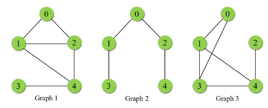
In this paper, the information exchange between agents is represented by an undirected switching topology network. The topology graphs are shown in Figure2. Correspondingly, the Laplacian matrices and the leader's adjacency matrices of each topology graph are given as
A discrete semi-Markov jump process with semi-Markov kernel is employed to describe the switching of topologies. The transition probability matrix of EMC and the probability density function of sojourn time are provided by
Let the upper bound of the sojourn-time for each topology mode be $$ T_{max}^{1}=T_{max}^{2}=T_{max}^{3}=5 $$. The statistical characteristic parameters of channel fading are selected as $$ \mu_{1}=0.8 $$, $$ \mu_{2}=0.7 $$, $$ \mu_{3}=0.75 $$, $$ \mu_{01}=0.75 $$, $$ \mu_{02}=0.85 $$, $$ \mu_{03}=0.6 $$, $$ \sigma_{1}=0.05 $$, $$ \sigma_{2}=0.15 $$, $$ \sigma_{3}=0.2 $$, $$ \sigma_{01}=0.1 $$, $$ \sigma_{02}=0.25 $$, $$ \sigma_{03}=0.15 $$.
First, we assume that there is no channel fading phenomenon between the leader and the follower, that is, $$ \xi_{op}(k)=1 $$ and $$ \varpi_{0p}(k)=0 $$ in system (6). In this case, mean square consensus conditions in Theorem 2 will be somewhat simplified. At this time, the channel interference between the follower and the follower is selected as
. The initial states of all agents and the initial mode of the communication topology are chosen as $$ x_{0}(0)=[0.2\; -0.1\; 0.2]^{T} $$, $$ x_{1}(0)=[0.1\; -0.3\; 0.4]^{T} $$, $$ x_{2}(0)=[-0.4\; 0.8\; -0.2]^{T} $$, $$ x_{3}(0)=[0.5\; -0.2\; 0.4]^{T} $$, $$ x_{4}(0)=[0.3\; -0.6\; -0.1]^{T} $$, and $$ \gamma(k)=1 $$.
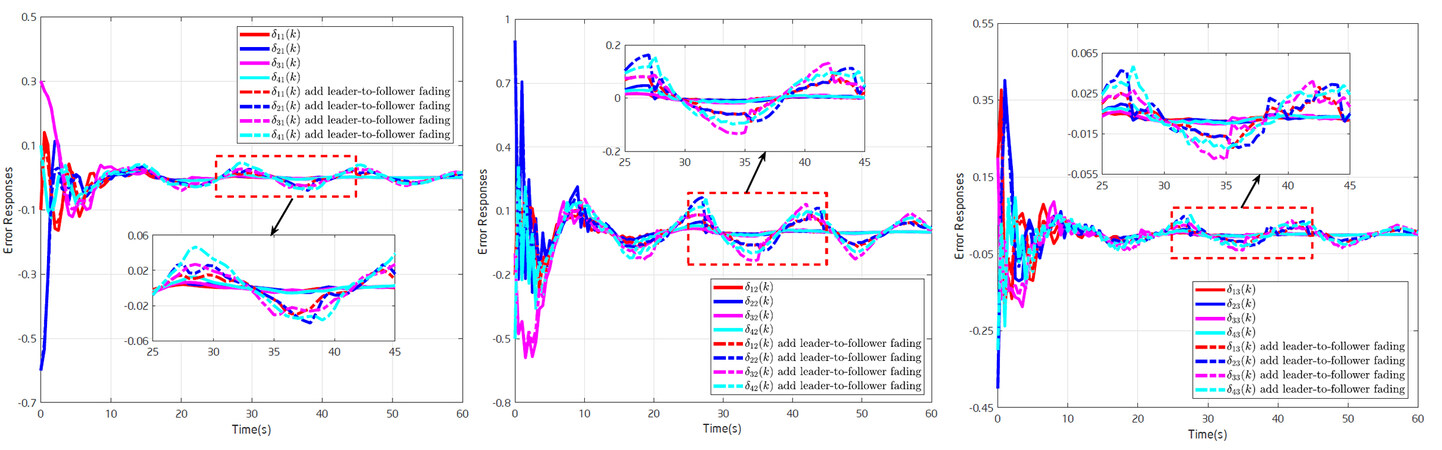
By solving simplified consensus conditions and simulating, we can obtain the state response curves of the system consensus error in this case as the solid line in Figure 3 shown. It shows that the controller designed in this paper is still effective when there is no fading phenomenon between the leader and follower agents. Then, the channel fading between the leader and the follower is added to the system under the condition that the controller remains unchanged, and the simulation experiment is performed again. The state trajectory of the consensus error is shown as the dotted line in Figure 3. The simulation results indicate that the fading phenomenon between the leader and the follower will affect the consensus and performance of the system. This further shows that it is necessary and meaningful to study the coexistence of the channel fading phenomenon between the leader and the follower, and the follower and the follower agent.
Figure 3. The consensus error responses under reduction conditions of Theorem 2 and additional leader-to-follower fading.
Next, consider the simultaneous existence of channel fading between leader and follower and between follower and follower. Choosing
. The rest of the parameters are the same as stated above. By solving the linear matrix inequality condition in Theorem 2, the controller gains $$ K_{p} $$ can be calculated as
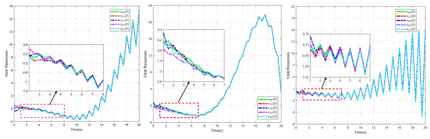
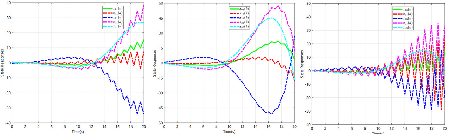
In addition, the $$ \mathcal{H}_{\infty} $$ performance index can be obtained as $$ \hat{\gamma}=2.3705 $$. According to Theorem 2, the state trajectories of all agents in the system (6) are shown in Figure 4. Figure 5 shows the state-response curves of each agent in the open-loop system. It can be seen that the designed control protocol (4) enables the system (6) to achieve leader-following mean square consensus under the premise of the simultaneous existence of channel fading and semi-Markov switching topologies.
Figure 4. The state responses of $$ x_{0}(k) $$ and $$ x_{i}(k) $$ under switching topologies $$ \mathcal{G}_{p} $$.
Figure 5. The state responses of $$ x_{0}(k) $$ and $$ x_{i}(k) $$ for the open-loop system.
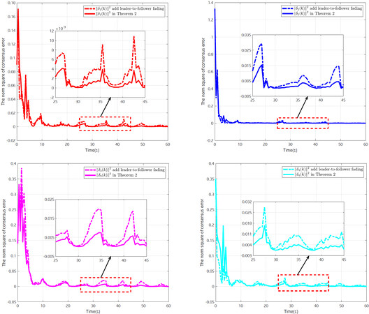
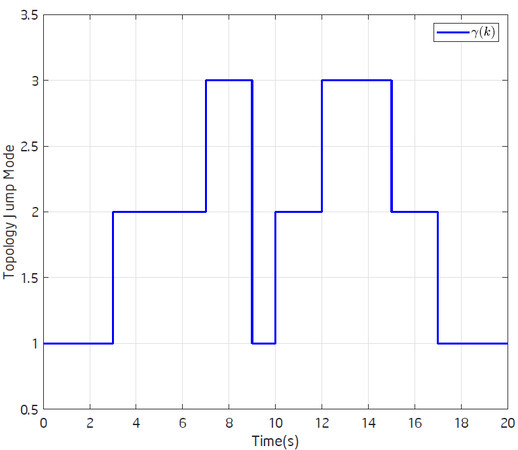
In Figure 6, the norm-squared response curves of consensus error in two different cases are given. One is the consensus error of the system in Theorem 2, and the other is the influence of channel fading on system performance when leader-to-follower fading is not considered. From the observation of Figure 6, we can find that the fluctuation of the norm-squared response curves for the consensus error in Theorem 2 represented by the solid line is weaker than that represented by the dotted line. The latter refers to the error norm squared response of the system suffering from leader-to-follower fading in Theorem 2 without considering leader-to-follower fading. This indicates that the consensus error of the former must stabilize faster than the latter. This further means that the control protocol proposed in this paper is more efficient and general. Figure 7 shows a possible topology jumping rule.
Figure 6. The norm-squared responses of $$ \delta_{i}(k) $$ under two different scenarios.
Figure 7. A possible mode jumping diagram of communication topologies.
Then, the relationship between the statistical properties of channel fading and the $$ \mathcal{H}_{\infty} $$ performance of the system (6) is discussed. We consider three different values for the variance of the channel fading coefficient variables $$ \xi_{p}(k) $$ and $$ \xi_{0p}(k) $$. By solving the conditions in Theorem 2, the value of the minimum $$ \hat{\gamma} $$ can be calculated and shown in Table 1. Table 1 lists three groups of simulation experiments. Simultaneously change the variance of one or two or three groups of fading coefficient variables and calculate the minimum performance index $$ \hat{\gamma} $$ of the system. It can be found from Table 1 that the greater the variance of the channel fading coefficient variables, the greater the $$ \mathcal{H}_{\infty} $$ performance index $$ \hat{\gamma} $$ of the system. At the same time, comparing the second experiment in the first group with the first experiment in the third group, as the number of variances increases, the $$ \mathcal{H}_{\infty} $$ performance index $$ \hat{\gamma} $$ of the system also increases. This means that the $$ \mathcal{H}_{\infty} $$ performance of the system will deteriorate as the effect of the fading channel on the transmitted signal or information becomes greater.
Table 1
$$ \mathcal{H}_{\infty} $$ performance with different values of variance for $$ \xi_{p}(k) $$ and $$ \xi_{0p}(k) $$
Number of variances $$\sigma_{p}$$ and $$\sigma_{0p}$$ that vary simultaneously
According to Table 2, it can be concluded that the consensus performance of the system will deteriorate or be destroyed, when Theorem 3.2 of[27], Theorem 3.2 of[41], and Simplified Theorem 2 in the absence of leader-to-follower fading additionally consider the channel fading of leader-to-follower. The control method proposed in Theorem 2 in this paper can still ensure the consensus performance of the system considering the channel fading between the leader-to-follower and follower-to-follower agents at the same time. This further proves that the model proposed in this paper is more general and the results are more effective than existing ones.
Table 2
Comparative simulations with literature [27, 41] for consensus performance
Method
Consensus performance under follower-to-follower fading
Consensus performance under leader-to-follower and follower-to-follower fading
Simplified Theorem 2 without leader-to-follower fading
Consensus
Consensus performance deterioration
Theorem 2
Consensus
Consensus
5. CONCLUSION AND FUTURE WORK
In this paper, the $$ \mathcal{H}_{\infty} $$ leader-following consensus problem of discrete multi-agent systems subject to channel fading is solved under switching topologies with semi-Markov kernel. First, a fading model that takes into account all inter-agent channels (including leader-to-follower channels) is established based on a discrete semi-Markov switching topology. Then, new sufficient criteria have been developed to ensure the mean-square stability and $$ \mathcal{H}_{\infty} $$ performance of the consensus error system (6) by means of stochastic analysis method and Lyapunov stability theory. Further, for the case where the semi-Markov kernel of switching topologies is not completely accessible, distributed consensus control protocols with fading states have been designed and the desired controller gains have been calculated based on linear matrix inequalities. Finally, a simulation example is presented to verify the effectiveness of the proposed approach. In future work, the problem of non-identical channel fading, adaptive fault-tolerant consensus and game optimization problems for heterogeneous or higher-order nonlinear multi-agent systems are interesting topics. In addition, how to reduce the number of decision variables in matrix inequality conditions and reduce the computational burden is also a problem worth studying.
DECLARATIONS
Authors' contributions
Made substantial contributions to the research, idea generation, algorithm design, simulation, wrote and edited the original draft: Yang H
Performed critical review, commentary and revision, as well as provided administrative, technical, and material support: Zhang H, Wang Z, Zhou X
Availability of data and materials
Not applicable.
Financial support and sponsorship
This work is supported by National Natural Science Foundation of China(61922063), Shanghai Hong Kong Macao Taiwan Science and Technology Cooperation Project (21550760900), Shanghai Shuguang Project (18SG18), Shanghai Natural Science Foundation(19ZR1461400), Shanghai Municipal Science and Technology Major Project (2021SHZDZX0100) and Fundamental Research Funds for the Central Universities. (Corresponding author: Zhang H).
Conflicts of interest
All authors declared that there are no conflicts of interest.
1. Dong X, Yu B, Shi Z, Zhong Y. Time-varying formation control for unmanned aerial vehicles: theories and applications. IEEE Trans Control Syst Technol 2015;23:340-8.
2. Dong X, Zhou Y, Ren Z, Zhong Y. Timevarying formation tracking for second-order multi-agent systems subjected to switching topologies with application to quadrotor formation flying. IEEE Trans Ind Electron 2016;64:5014-24.
3. Kladis GP, Menon PP, Edwards C. Fuzzy distributed cooperative tracking for a swarm of unmanned aerial vehicles with heterogeneous goals. Int J Syst Sci 2016;47:3803-11.
4. El-Ferik S, Elkhider SM, Ghommam J. Adaptive containment control of multi-leader fleet of underwater vehicle-manipulator autonomous systems carrying a load. Int J Syst Sci 2019;50:1501-16.
5. Do KD. Synchronization motion tracking control of multiple underactuated ships with collision avoidance. IEEE Trans Ind Electron 2016;63:2976989.
6. Li X, Dong X, Li Q, Ren Z. Event-triggered time-varying formation control for general linear multi-agent systems. J Franklin Inst 2019;356:10179-95.
7. Su H, Zhang J, Chen X. A stochastic sampling mechanism for time-varying formation of multiagent systems with multiple leaders and communication delays. IEEE Trans Neural Netw Learn Syst 2019;30:3699-3707.
8. Ding C, Dong X, Shi C, Chen Y, Liu Z. Leaderless output consensus of multi-agent systems with distinct relative degrees under switching directed topologies. IET Control Theory A 2018;13:313-20.
9. Gao R, Huang J, Wang L. Leaderless consensus control of uncertain multi-agents systems with sensor and actuator attacks. Inf Sci 2019;505:144-56.
10. Cui Q, Huang J, Gao T. Adaptive leaderless consensus control of uncertain multiagent systems with unknown control directions. Int J Rob Nonl Control 2020;30:6229-40.
11. Chen C, Lewis F L, Li X. Event-triggered coordination of multi-agent systems via a Lyapunov-based approach for leaderless consensus. Automatica 2022;136:109936.
12. He W, Lv S, Wang X, Qian F. Leaderless consensus of multi-agent systems via an event-triggered strategy under stochastic sampling. J Franklin Inst 2019;356:6502-24.
13. He X, Wang Q. Distributed finite-time leaderless consensus control for double-integrator multi-agent systems with external disturbances. Appl Math Comput 2017;295:65-76.
14. You X, Hua C, Yu H, Guan X. Leader-following consensus for high-order stochastic multi-agent systems via dynamic output feedback control. Automatica 2019;107:418-24.
15. Liu W, Huang J. Leader-following consensus for linear multiagent systems via asynchronous sampled-data control. IEEE Trans Automat Contr 2019;65:3215-22.
16. Liu J, Yin T, Yue D, Karimi H R, Cao J. Event-based secure leader-following consensus control for multiagent systems with multiple cyber attacks. IEEE Trans Cybern 2020;51:162-73.
17. Shang Y, Ye Y. Leader-follower fixed-time group consensus control of multiagent systems under directed topology. Complexity 2017;2017:1-9.
18. Zhang D, Deng C, Feng G. Resilient cooperative output regulation for nonlinear multi-agent systems under DoS sttacks. IEEE Trans Automat Contr 2022;Early Access.
19. Zhang D, Deng C, Feng G. Resilient practical cooperative output regulation for MASs with unknown switching exosystem dynamics under DoS attacks. Automatica 2022;139:110172.
20. Zhang D, Ye Z, Dong X. Co-design of fault detection and consensus control protocol for multi-agent systems under hidden DoS attack. IEEE Trans Circuits Syst 2021;68:2158-70.
21. Wang J, Wang Y, Yan H, Cao J, Shen H. Hybrid event-based leader-following consensus of nonlinear multiagent systems with semi-Markov jump parameters. IEEE Syst J 2020;16:397-408.
22. Zhang Z, Su S, Niu Y. Dynamic event-triggered control for interval type-2 fuzzy systems under fading channel. IEEE Trans Cybern 2020;51:5342-51.
23. Li X, Zhang B, Li P, Zhou Q, Lu R. Finite-horizon $$H_{\infty}$$ state estimation for periodic neural networks over fading channels. IEEE Trans Neural Netw Learn Syst 2019;31:1450-1460.
24. Elia N. Remote stabilization over fading channels. Systems and Control Letters 2005;54:237-49.
25. Yan H, Zhang H, Yang F, Zhan X, Peng C. Event-triggered asynchronous guaranteed cost control for Markov jump discrete-time neural networks with distributed delay and channel fading. IEEE Trans Neural Netw and Learn Syst 2018;29:3588-98.
26. Xiao N, Xie L, Qiu L. Feedback stabilization of discrete-time networked systems over fading channels. IEEE Trans Automat Contr 2012;57:2176-89.
27. Gu X, Jia T, Niu Y. Consensus tracking for multi-agent systems subject to channel fading: A sliding mode control method. Int J Syst Sci 2020;51:2703-11.
28. Xu L, Xiao N, Xie L. Consensusability of discrete-time linear multi-agent systems over analog fading networks. Automatica 2016;71:292-9.
29. Xu L, Zheng J, Xiao N, Xie L. Mean square consensus of multi-agent systems over fading networks with directed graphs. Automatica 2018;95:503-10.
30. Liu Z-W, Wen G, Yu X, Guan Z-H, Huang T. Delayed impulsive control for consensus of multiagent systems with switching communication graphs. IEEE Trans Cybern 2020;50:3045-55.
31. Jiang J, Jiang Y. Leader-following consensus of linear time-varying multi-agent systems under fixed and switching topologies. Automatica 2020;113:108804.
32. Li B, Wen G, Peng Z, Huang T, Rahmani A. Fully distributed consensus tracking of stochastic nonlinear multiagent systems with Markovian switching topologies via intermittent control. IEEE Trans Syst, Man, Cybern: Syst 2021;52:3200-9.
33. Shang Y. Couple-group consensus of continuous-time multi-agent systems under Markovian switching topologies. J Franklin Inst 2015;352:4826-44.
34. Ge X, Han Q. Consensus of multiagent systems subject to partially accessible and overlapping Markovian network topologies. IEEE Trans Cybernet 2017;47:1807-19.
35. Dai J, Guo G. Event-triggered leader-following consensus for multi-agent systems with semi-Markov switching topologies. Inf Sci 2018;459:290-301.
36. Li K, Mu X. Containment control of stochastic multiagent systems with semi-Markovian switching topologies. Int J Rob Nonlin Contr 2019;29:4943-55.
37. Liang H, Zhang L, Sun Y, Huang T. Containment control of semi-Markovian multiagent systems with switching topologies. IEEE Trans Syst, Man, Cybernet: Syst 2019;51:3889-99.
38. He M, Mu J, Mu X. $$H_{\infty}$$ leader-following consensus of nonlinear multi-agent systems under semi-Markovian switching topologies with partially unknown transition rates. Infor Sci 2020;513:168-79.
39. Zhang L, Leng Y, Colaneri P. Stability and stabilization of discrete-time semi-Markov jump linear systems via semi-Markov kernel approach. IEEE Trans Automat Contr 2016;61:503-8.
40. Ning Z, Zhang L, Colaneri P. Semi-Markov jump linear systems with incomplete sojourn and transition information: Analysis and synthesis. IEEE Trans Automat Contr 2020;65:159-74.
41. Li W, Niu Y, Cao Z. Event-triggered sliding mode control for multiagent systems subject to channel fading. Int J Syst Sci 2021;53:1233-44.
Yang H, Zhang H, Wang Z, Zhou X. ℋ∞ leader-following consensus of multi-agent systems with channel fading under switching topologies: a semi-Markov kernel approach. Intell Robot 2022;2(3):223-43. http://dx.doi.org/10.20517/ir.2022.19
AMA Style
Yang H, Zhang H, Wang Z, Zhou X. ℋ∞ leader-following consensus of multi-agent systems with channel fading under switching topologies: a semi-Markov kernel approach. Intelligence & Robotics. 2022; 2(3): 223-43. http://dx.doi.org/10.20517/ir.2022.19
Chicago/Turabian Style
Yang, Haoyue, Hao Zhang, Zhuping Wang, Xuemei Zhou. 2022. "ℋ∞ leader-following consensus of multi-agent systems with channel fading under switching topologies: a semi-Markov kernel approach" Intelligence & Robotics. 2, no.3: 223-43. http://dx.doi.org/10.20517/ir.2022.19
ACS Style
Yang, H.; Zhang H.; Wang Z.; Zhou X. ℋ∞ leader-following consensus of multi-agent systems with channel fading under switching topologies: a semi-Markov kernel approach. Intell. Robot.2022, 2, 223-43. http://dx.doi.org/10.20517/ir.2022.19
Comments must be written in English. Spam, offensive content, impersonation, and private information will not be permitted. If any
comment is reported and identified as inappropriate content by OAE staff, the comment will be removed without notice. If you have any
queries or need any help, please contact us at
support@oaepublish.com.

 0
0 , ...
, ... 


 Cite This Article 12 clicks

 Like This Article 21
likes
Like This Article 21
likes


Comments
Comments must be written in English. Spam, offensive content, impersonation, and private information will not be permitted. If any comment is reported and identified as inappropriate content by OAE staff, the comment will be removed without notice. If you have any queries or need any help, please contact us at support@oaepublish.com.