A node selection algorithm to graph-based multi-waypoint optimization navigation and mapping

1. INTRODUCTION

Robotics system has been applied to numerous fields, such as transportation ^[1], healthcare service ^{[2, 3]}, agriculture ^[4], manufacturing ^[5], etc., in recent years. Robot navigation is one of the fundamental components in robotic systems, which includes multi-waypoint navigation system ^[6-8]. As an increasing demand and limited onboard resources for autonomous robots, it requires the ability to visit several targets in one mission to optimize multiple objectives, including time, robot travel distance minimization, and spatial optimization ^[9-15]. For example, due to a global pandemic, the world struggled to sanitize heavily populated areas, such as airports, hospitals, and educational buildings. Autonomous robots with multi-waypoint navigation systems can effectively sanitize all targeted areas without endangering the workers ^{[14, 16]}. As well as in agriculture management, multi-waypoint strategies allow the robotic system to navigate and survey multiple areas to assist in production and collection.

In order to employ robotic systems in real-world scenarios, one critical factor is to develop autonomous robot multi-waypoint navigation and mapping system ^[17]. In order to solve the autonomous robot navigation problem, countless algorithms have been developed, such as graph-based^{[18, 19]}, ant colony optimization (ACO) ^[20-22], bat-pigeon algorithm (BPA) ^[23], neural networks ^[24-26], fuzzy logic ^[27], artificial potential field (APF) ^[28], sampling-based strategy ^{[14, 29]}, hybrid algorithms^[30], task planning algorithm ^[31], etc. Chen et al. produced a hybrid graph-based reinforcement learning architecture to develop a method for robot navigation in crowds ^[18]. Luo et al. proposed an improved vehicle navigation method, which utilizes a heading-enabled ACO algorithm to improve trajectory towards the target^[20]. Lei et al. developed a Bat-Pigeon algorithm with the ability to adjust the speed navigation of autonomous vehicles ^[23]. Luo et al. developed the model for multiple robots complete coverage navigation while using a bio-inspired neural network to dynamically avoid obstacles^[32]. Na and Oh established a hybrid control system for autonomous mobile robot navigation that utilizes a neural network for environment classification and behavior-based control method to mimic the human steering commands^[25].Lazreg and Benamrane ^[27] developed a neuro-fuzzy inference system associated with a Particle Swarm Optimization (PSO) method for robot path planning using a variety of sensors to control the speed and position of a robot.Jensen-Nau et al.^[28] integrated a Voronoi-based path generation algorithm and an artificial potential field path planning method, in which the latter is capable of establishing a path in an unknown environment in real-time for robot path planning and obstacle avoidance.Penicka and Scaramuzza ^[14] developed a sampling-based multi-waypoint minimum-time path planning model that allows obstacle avoidance in cluttered environments.Ortiz and Yu ^[30] proposed a sliding control method in combination with simultaneous localization and mapping (SLAM) method to overcome the bounded uncertainties problem, which utilizes a genetic algorithm to improve path planning capabilities. Bernardo et al. proposed a task planning method for home environment ontology to translate tasks given by other robots or humans into feasible tasks for another robot agent^[31].

In robotic path planning, one of the special topics is autonomous robot multi-waypoint navigation which has been studied for many years. For instance, Shair et al. proposed a model for real-world waypoint navigation using a variety of sensors for accurate environmental analysis^[33]. The system is designed utilizing the wide area augmentation system (WAAS) and the European geostationary navigation overlay service (EGNOS) for GPS in combination with aerial images to provide valuable positioning data to the system.Yang ^[34] brought about a multi-waypoint navigation system based on terrestrial signals of opportunity (SOPs) transmitters, which has the ability to operate in environments that are not available to global navigation satellite systems (GNSS) for unmanned aerial vehicles (UAV).Janoš et al. proposed a sampling-based multi-waypoint path planner, space-filling forest method to solve the problem of finding collision-free trajectories while the sequence of waypoints is formed by multiple trees^[29].However, the aforementioned approaches have not taken into account the safety of the robot during navigation. In real-world applications, an autonomous vehicle has odometry errors during operation. The safety-aware road model is developed utilizing the Generalized Voronoi diagram (GVD) approach. Once the safety-aware roads are defined, a particle swarm optimization (PSO) algorithm-based multi-waypoint path planning algorithm is proposed to visit each waypoint in an explicated sequence while simultaneously avoiding obstacles. In this paper, the Adjacent Node Selection (ANS) algorithm is developed to select the closest nodes on the safety-aware roads to generate the final collision-free trajectories with minimal distance. Furthermore, in our hybrid algorithm, we utilize a histogram-based reactive local navigator to avoid dynamic and unknown obstacles within the workspace. Through all of these methods, an effective and efficient safety-aware multiple waypoint navigation model was established, which has been validated by both simulations and comparison studies.

This paper proposes an Adjacent Node Selection (ANS) algorithm for obtaining an optimal access node into graph-based maps. To the best of our knowledge, there are no known similar algorithms that improve the paths created from the waypoint to the graph. The ANS algorithm can be applied to any graph-based mapping environment, which improves the various graph-based models used for autonomous robotic path planning systems. In finding an access point into the graph utilizing one of the nodes in the system, the ANS algorithm conducts point-to-point selection in dense obstacle field of environments to obtain a node to gain access to the graph that forms a resumable path from a waypoint to the graph. The algorithm's overall goal is to find a node in a graph-based map and shorten the overall path length from each waypoint to waypoint, and the waypoint to the graph.

One can see in Figure 1 the overall framework of our proposed model. Initially, the model is provided with a global map of its environment and the location of each target waypoint. The GVD utilizes the global map to construct the safety-aware roads, which are used to guide the robot throughout the environment. The targeted waypoint locations are used as input to the improved PSO (IPSO) algorithm that act as our waypoint sequencing module, which is utilized to find a near-optimal sequence to visit each waypoint. The ANS algorithm utilizes the output from the previous stages. The ANS algorithm finds the best node for each waypoint to use as an access point to the graph. If there is no direct path from one waypoint to a node in the graph, the algorithm conduces point-to-point navigation with nodes within a specified range, which will be explained in later sections of the paper. Once each waypoint has found its access point, the safety-aware path is constructed, which is then applied to our path smoothing algorithm. Finally, we utilize a reactive local navigation system to detect obstacles autonomously and simultaneously build a map of the environment along the generated path.

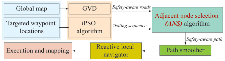
Figure 1. Illustration of the proposed model framework.

The main contributions of this paper with this framework of concurrent multi-waypoint navigation and mapping with collision avoidance as are summarized as follows: (1) An adjacent node selection (ANS) algorithm is proposed to build up regional bridges from waypoints to nodes or edges on the graph in multi-waypoint navigation and mapping; (2) a concurrent multi-waypoint navigation and mapping framework of an autonomous robot is developed by the generalized Voronoi diagram (GVD) and IPSO algorithm as well as a local navigator; (3) a GVD method is employed to plan safety-aware trajectories in an obstacle populated environment, while the sequence of multiple waypoints is created by the IPSO algorithm to minimize the total distance cost; (4) a sensor-based histogram robot reactive navigator coupled with map building is adopted for moving obstacle avoidance and local mapping. An improved $$\mathcal{B}$$-spline curve-based speed modulation module is adopted for smoother navigation.

The structure of this paper is as follows. Section II presents the safety-aware model that constructs the safety-conscious roads for robot traversal. Section III describes the proposed adjacent node selection algorithm to find an access node into the graph-based map. Section IV, the improved PSO-based (IPSO) multi-waypoint navigation model for waypoint sequencing is explained. Section V illustrates the reactive local navigator for real-time workspace building and obstacle avoidance. Section VI depicts simulation results and comparative analyses. Several important properties of the proposed framework are summarized in Section VII.

2. SAFETY-AWARE MODEL

Computational geometry has exceedingly studied the Voronoi diagrams (VD) model, which is an elemental data structure used as a minimizing diagram of a finite set of continuous functions ^{[28, 35]}. The minimized function defines the distantance to an object within the workspace. The VD model decomposes the workspace into several regions, each consisting of the points near a given object than the others. Let $$ \mathcal{G} = \{g_1\cdots, g_n\} $$ be a set of points of $$ \mathbb{R}^d $$ to each $$ g_i $$ associated with a specific Voronoi region $$ V(g_i) $$. This can be expressed by the following equation^{[36, 37]}:

The intersection of $$ n - 1 $$ half spaces can be denoted by the region $$ V(g_i) $$. Each half space holds a point $$ g_i $$ along with another point of $$ \mathcal{G} $$. The regions $$ V(g_i) $$ are convex polyhedrons due to the bisectors acting as hyperplanes between each region. The generalized Voronoi diagram (GVD) is a modified version of the VD model defined as the set of points Euclidean distance from two obstacles^[37]. The workspace is represented as a graph by the GVD model consisting of nodes, edges, and vertices ^[28].

The proposed ANS algorithm utilizes nodes and edges obtained from the GVD illustrated in Figure 2A. The nodes in the GVD act as junctions to connect waypoints, whereas the edges are used to determine the search range in view of waypoints. Solely the nodes in the search range are calculated, other than the entire workspace, thus reducing the computational expense. Figure 2B reveals that the range of some edges fails to evaluate how spare of the workspace is configurated. These edges with short lengths are distractors for evaluating and computing the search range, thus need to be eliminated shown in Figure 2B. In our ANS algorithm, those edges with the shortest 10% are eliminated, while the rest of the edges are averaged to compute the radius of the search range. One circumstance is exhibited in Figure 2C, in which some nodes fail to fall into the search range once the excessively short edges are excluded. The original search space in solid circles and modified search space in dashed circles based on the ANS algorithm are shown in Figure 2C. As may be seen, after excessively short edges are effectively eliminated, an appropriate search range is achieved.

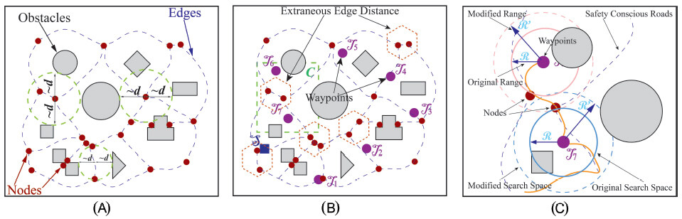
Figure 2. Illustration of the ANS algorithm and the safety-aware model by creation of the GVD. (A) Depicts the equidistance property of the nodes and edges in the GVD model. (B) illustrates how we remove extraneous edge distances, which are small edges within the graph that reduce the search space or range in the ANS algorithm. (C) illustrates how the removal of those extraneous edges improves the range and how an access node to the graph can be found.

GVD nodes form the Euclidean distance between two or more obstacles, while the edges are the junction of two nodes that depict the distance between each neighboring node to another. Vertices are the connection points between three or more nodes. Using these features from the GVD model, an obstacle-free path with our safety-aware model is effectively created. The safety-aware model is constructed by inputting an image and extracting all significant features from the image, thus allowing the model to construct a map from the input image. The safety-aware roads are the clearest path between obstacles that occupy the available space in the map, which can be seen in Figure 2.

In this paper, in order to explain our proposed ANS algorithm, how the nodes are determined and constructed with the GVD will be presented in some detail. We will introduce some definitions and notations. Lee and Drysdale ^[36] derive four basic definitions for determining the optimal placement of edges and nodes within the GVD graph.

DEFINITION 1. A closed line segment $$ M $$ consists of two endpoints $$ \alpha $$ and $$ \gamma $$. A straight line is denoted by ($$ \alpha $$, $$ \gamma $$), which is also known as an open segment. Elements within the derivation are referred to as points or segments. The straight line containing $$ M $$ is denoted by $$ \overleftrightarrow{M} $$. The same line directed from $$ \alpha $$ to $$ \gamma $$ is denoted by $$ \vec M $$.

DEFINITION 2. The projection $$ \sigma(\epsilon, M) $$ of a point $$ q $$ onto a closed segment $$ M $$, is the intersection of $$ \overleftrightarrow{M} $$ and is perpendicular to $$ M $$ and passing through $$ \epsilon $$.

DEFINITION 3. The distance between $$ \omega (\epsilon, M) $$ is a point $$ \epsilon $$ and a closed segment $$ M $$ in the Euclidean metric is defined as the distance $$ \omega(\epsilon, \sigma(\epsilon, M)) $$ between the point $$ \epsilon $$ and its projection onto $$ M $$ if $$ \sigma(\epsilon, M)) $$ belongs to $$ M $$ and is $$ \min $$$$ (\omega(\epsilon, \alpha), \omega(\epsilon, \gamma)) $$ otherwise. In other words, $$ \omega(\epsilon, M) = $$$$ \min_{u \in M} (\epsilon, u ) $$. The point of $$ M $$, which is closest to $$ \epsilon $$, is called the image $$ I(\epsilon, M) $$ of $$ \epsilon $$ on $$ M $$.

DEFINITION 4. The bisector $$ \beta(c_{i}, c_{j}) $$ of two elements {$$ c_{i} $$ and $$ c_{j} $$} is the locus of points equidistant from $$ c_{i} $$ and $$ c_{j} $$. The bisector $$ \beta(Z, Q) $$ of two sets of elements $$ Z $$ and $$ Q $$ is defined to be the locus of points equidistant from $$ Z $$ and $$ Q $$, where the distance $$ \omega(\epsilon, Z) $$ between a point $$ \epsilon $$ and a set of elements $$ Z $$ is defined to be $$ \min_{c \in Z}\omega(\epsilon, c ) $$. The bisector $$ \beta(c_{i}, c_{j}) $$ is said to be oriented if a direction is imposed upon it so that elements $$ c_{i} $$ and $$ c_{j} $$ lie to the left and the right of it, respectively. An oriented bisector $$ \beta(Z, Q) $$ is defined similarly.

Utilizing these four definitions, we can easily establish {edges} {among} spaces or obstacles, which uses the equidistant to create an optimal edge that lies directly between the two spaces. As seen in the above {definitions, } we can also create edges between irregular-shaped spaces {and} obstacles.

To characterize the GVD, we expect the robot to be operated at a point within the workspace, a $$ W $$, which is populated by convex obstacles $$ C_{1}, . . . , C_{n} $$. Non-convex obstacles are displayed as the union of convex shapes. The distance between a point and an obstacle is the minimal distance between the point and all points of the obstacle. The distance function, and its "gradient" are represented as:

where in Equation (2) $$ d_i $$ is the distance to obstacle $$ C_i $$ from a point $$ x $$, and in Equation (3) $$ \nabla d_i(x) $$ is the unit vector in the direction from $$ x $$ to $$ c_0 $$, where $$ c_0 $$ is the closest point to $$ x $$ in $$ C_i $$. The essential structure block of the GVD is the arrangement of points equidistant to two sets $$ C_i $$ and $$ C_j $$, with the end goal that each set in this set is the minimal distance to the obstacles $$ C_i $$ and $$ C_j $$ than other obstacles. This type of structure is known as the two-equidistant face,

Each face has a co-dimension in the ambient space, which causes the two-equidistant faces to be seen as one-dimensional. The intersection of both faces forms the GVD and is denoted by the following equation:

3. ADJACENT NODE SELECTION ALGORITHM

The details of the adjacent node selection algorithm are shown in Figure 3. Within the search range obtained, we applyIPSO-based path planning algorithm to generate the connection path from the waypoint to all the potential nodes in the range. The connection path is planned in the grid-based map as shown in Figure 3A. The search range in the larger map is shown in Figure 3B, which is also a part of Figure 6. Finally, with the formation of a collision-free path to the adjacent nodes from the two waypoints, we obtain the optimal path selection by calculating the overall path length $$ \mathcal{L}_{c} + \mathcal{L}_{e} $$.

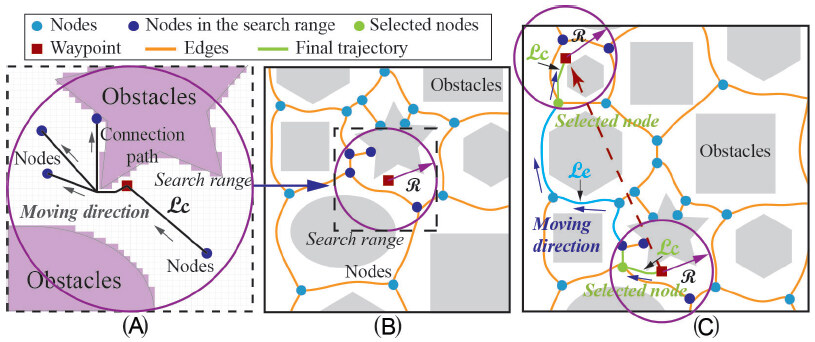
Figure 3. Details of the Adjacent Node Selection (ANS) algorithm. (A) The IPSO-based connection path planning in the search range. (B) The search range determination and node selection inside. (C) The final generated path with the minimum path length.

To show the necessity of IPSO-based path planning from waypoints to adjacent nodes, a more specific scenario is shown in Figure 4. In Figure 4A, all straight lines connecting nodes and waypoints are separated by obstacles. Among them, points $$ i $$ and point $$ j $$ are located in our search range. If we only rely on the Euclidean distance between node and waypoint, it can be found that the point $$ i $$ is closer to the waypoint. However, after considering the path with obstacle avoidance, the path for point $$ i $$ to the waypoint is longer. To sum up, the obtained search range with ANS algorithm and the IPSO-based path planning algorithm can reduce the computational cost while ensuring a short and safe trajectory. The details of the procedure are described in Algorithm 2.

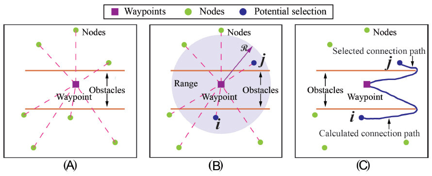
Figure 4. Illustration of ANS method within a more specific sense, where an obstacle obstructing the connection path. (A) The multiple connection paths have been obstructed by the obstacles. (B) It selects the nodes in the defined range. (C) It conducts IPSO point-to-point algorithm to achieve the optimal path to the selected node.

We carry out further discussions on our proposed ANS algorithm. Figure 5A and Figure 5B are parts of Figure 11 and Figure 13 (enclosed in pink dashed boxes), respectively. As shown in Figure 5A, the solid circles represent the search radius of the waypoints in the simulation and the red solid dots depict the nodes in the workspace. In Figure 11, we end up with the trajectory that follows the generated safe-aware road. However, if the space in the map is more sparse, our search radius $$ \mathcal{R} $$ may increase to $$ \mathcal{R}' $$, which may achieve the waypoints in their respective search spaces. Thus, instead of following the safe-awareness road, a new connection path is obtained through the improved PSO algorithm directly, as shown in dashed lines in Figure 5A. Moreover, the sparseness of the overall workspace may not represent the complexity of local obstacles. Therefore, the choice of the radius of the search space may require more mathematical proof and analysis.

Figure 5. Illustration of the ANS algorithm analysis. (A) From Figure 11 it is enclosed by a pink dashed box. (B) From Figure 13 it is enclosed by a pink dashed box.

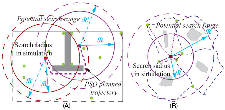
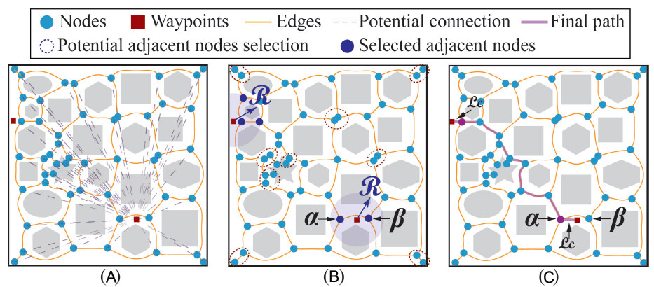
Figure 6. Illustration of the Adjacent Node Selection (ANS) algorithm. (A) The workspace with nodes, edges and waypoints. (B) The node selection in the search range. (C) The final generated path.

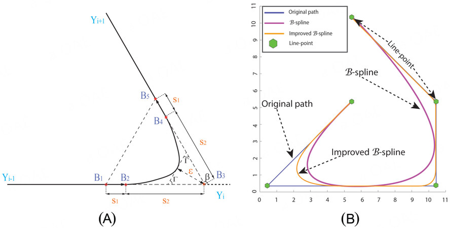
Figure 7. Illustration of the B-spline function. (A) The improved segmented B-spline curve. (B) The same path smoothed by the fundamental B-spline and the improved B-spline function.

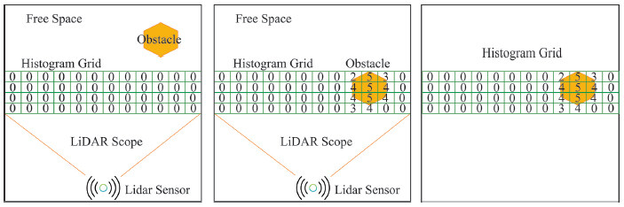
Figure 8. Illustration of how the VHF uses a probability along with histogram-based grid to detect and build a map simultaneously.

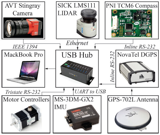
Figure 9. Robot sensor configuration for multi-waypoint navigation and mapping.

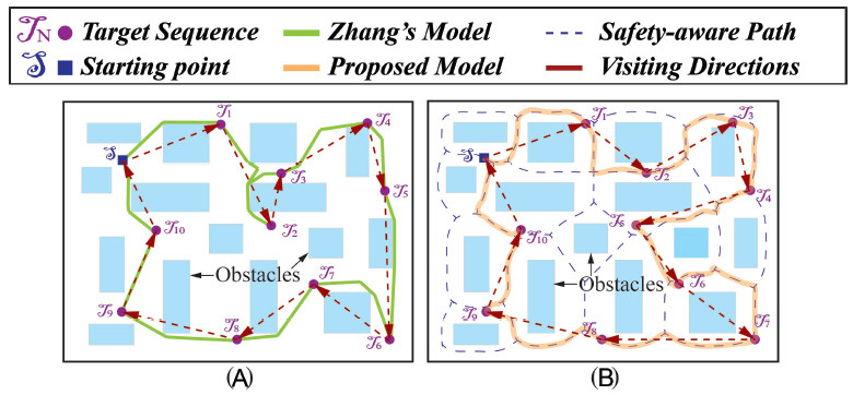
Figure 10. Illustration of the path created from the other models^[43]. (A) It depicts the path created by Zhang et al.'s model by the green lines (redrawn by Zhang et al., 2021^[43]). (B) It represents the proposed method point order and traversed path. The point order is illustrated by the violet arrows, while the orange path represents the robot path. Safety-aware roads are depicted by the blue dashed lines. The waypoints are illustrated by the violet circles.

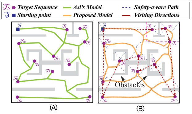
Figure 11. Illustration of the path created from the other models^[44]. (A) It depicts the path created by Asl and Taghirad model by the green lines (redrawn by Asl and Taghirad, 2019^[44]). (B) It represents the proposed method point order and traversed path. The point order is illustrated by the violet arrows, while the orange path represents the robot path. Safety-aware roads are depicted by the blue dashed lines. The waypoints are illustrated by the violet circles.

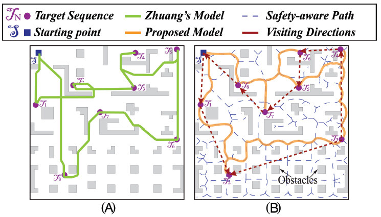
Figure 12. Illustration of the path created from the compared models^[45]. (A) It depicts the path created by Zhuang et al.'s model by the green lines (redrawn from Zhuang et al., 2021^[45]). (B) It represents the proposed method point order and traversed path. The point order is illustrated by the violet arrows, while the orange path represents the robot path. Safety-aware roads are depicted by the blue dashed lines. The waypoints are illustrated by the violet circles.

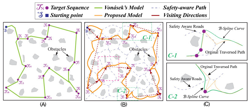
Figure 13. Illustration of the path created from the compared models^[46]. (A) It depicts the path created by Vonásek's model shown by the green lines (redrawn from Vonásek and Penicka, 2019^[46]). (B) It represents the proposed method point order and traversed path. The point order is illustrated by the violet arrows, while the orange path represents the robot path. Safety-aware roads are depicted by the blue dashed lines. The waypoints are illustrated by the violet circles. (C) It depicts how the B-spline curve is applied to the known path, which smooths and reduces the path for a local navigator to traverse.

With the increasing radius of the potential search range, more nodes are applicable for selection, such as the nodes connected with dashed lines in Figure 5B. Enlarging the search space may avoid some unnecessary detours and give a shorter path. Therefore, the trade-off between path length and safety of the autonomous robot still requires more consideration.

4. IMPROVED PSO-BASED MULTI-WAYPOINT NAVIGATION

The particle swarm optimization (PSO) algorithm is a swarm-based bio-inspired algorithm based on the behavioral observation of birds. It uses an iterative methodology to optimize randomly initialized particles to define a path from the initial position to the goal ^[27]. In this section an improved PSO (IPSO) algorithm by introduction of a weighted particles is addressed to resolve the multi-waypoint sequence issue.

4.1. Multi-waypoint visiting sequence

In real-world scenarios, one important factor is that the GPS coordinates provide portions for the multiple waypoints. Traveling from one waypoint to another, the distance between them determines their associated cost. The primary purpose of traveling from one waypoint to another is to simultaneously find the minimal cost of all generated trajectories. Using the coordinates of each waypoint and the PSO algorithm, the minimal-distance path can be found within the environment. The PSO algorithm finds the best waypoint visiting sequence by initializing randomized particles. The algorithm denotes the local best position as {$$ x^b $$} and the global best position as {$$ x^g $$}. Then by taking advantage of a fitness function, the algorithm guides each particle towards the local and global best positions. The particle velocities are updated as follows:

(6) $$ \begin{equation} \begin{array}{l} v_{p}(t+1)=v_{p}(t)+ \alpha_{1}\omega_{1}[ {x^b_{p}(t)}-x_{p}(t)]+ \alpha_{2}\omega_{2}[ {x^g_{p}(t)}-x_{p}(t)] \end{array} \end{equation} $$

(7) $$ \begin{equation} \begin{array}{l} {x_{p}^{(t+1)}=x_{p}^{(t)}+ v_{p}^{(t+1)}} \end{array} \end{equation} $$

where, $$ v_p(t) $$ represents the velocity of particle $$ p $$ at instant $$ t $$, {$$ x_p(t) $$} is the position of particle $$ p $$ at instant $$ t $$, $$ \alpha_{1} $$ and $$ \alpha_{2} $$ are the positive acceleration constants used to scale the contribution of cognitive and social components. $$ \omega_{1} $$ and $$ \omega_{2} $$ are the uniform random number between 0 and 1. {$$ x^b_p(t) $$} is the best position the particle $$ p $$ achieved up to instant $$ t $$ at current iteration, {$$ x^g_p(t) $$} is the {global} position that any of $$ p $$'s neighbors has reached up to instant $$ t $$. However, if a particle $$ p_i $$ lies close to the $$ x^b_p(t) $$ and $$ x^g_p(t) $$, only one term guides the $$ p_i $$ to search the potential solution.The optimization process in our navigation issue is more likely trapped in local minima. Thus, an improved PSO algorithm is utilized to provide a more promising search direction for all particles during the optimization process.

(8) $$ \begin{equation} x^{w}=\sum\limits_{i=1}^{P} \bar{\alpha}_{i}^{w} {x^b_i(t)} \end{equation} $$

(9) $$ \begin{equation} \bar{\alpha}_{i}^{W}=\frac{\hat{\alpha}_{i}^{W}}{\sum_{j=1}^{P} \hat{\alpha}_{i}^{W}} \end{equation} $$

(10) $$ \begin{equation} \begin{aligned} &\hat{\alpha}_{i}^{W}=\frac{\max _{1 \leq k \leq M}\left(\mathcal{F}\left( {x^b_k(t)}\right)\right)-\mathcal{F}\left( {x^b_i(t)}\right)+\varepsilon}{\max _{1 \leq k \leq M}\left(\mathcal{F}\left( {x^b_k(t)}\right)\right)-\min _{1 \leq k \leq M}\left(\mathcal{F}\left( {x^b_k(t)}\right)\right)+\varepsilon}, \quad i=1, 2, \ldots, M, \end{aligned} \end{equation} $$

where $$ \varepsilon $$ is a positive constant, $$ \hat{\alpha} $$ is the weighted constant of each particle. $$ \mathcal{F}(\cdot) $$ is the fitness function. The worst and the best fitness values of all personal best particles are represented by $$ \max _{1 \leq k \leq M}(\mathcal{F}\left(x_{k}^{P}\right)) $$ and $$ \min _{1 \leq k \leq M}(\mathcal{F}\left(x_{k}^{P}\right)) $$, respectively.

The order is optimized through this method, in which each waypoint is visited. A sequence of particles are initialized to compose a population in the original PSO algorithm. A possible optimal solution to an optimization issue in our multi-waypoint sequence is discovered by one particle in the PSO. This particle indicates a possible optimal solution to the multi-waypoint navigation issue and moves to explore an optimal solution in a certain search space. In this paper, a weighted particle is introduced into a swarm to suggest a more reasonable search direction for all the particles. As a result, the best position of particle and neighbor guides the particle to move along the corrected direction for better covergence.

The multi-waypoint visiting sequence problem can be used to solve the transportation planning problem and Covid-19 disinfection robot path planning in hospitals, in which agents (vehicles) need to be delivered as well as the overall cost and time need to be minimized ^[14]. The algorithm of the improved PSO to finding multi-waypoint visiting sequence is explained in Algorithm 1. The objective of the algorithm is to minimize the total trajectory length of Cartesian coordinates $$ (X_n, Y_n) $$ of waypoints given.

In the IPSO model the $$ \mathcal{P}_A $$ represents the particle agent, which is denoted by the $$ \mathcal{P}_A $$ : {$$ \mathcal{P}_b $$, $$ \mathcal{P}_g $$, $$ \mathcal{N} $$}. $$ \mathcal{N} $$ holds a group of particle agents which are predetermined as neighbors of $$ \mathcal{P}_A $$. The $$ \mathcal{P}_A $$ are defined by the following parameters.

(1) Each $$ \mathcal{P}_A $$ requests each neighbor's current personal best location.

(2) Each $$ \mathcal{P}_A $$ returns its current personal best to neighbors.

(3) Obtains the center location of each surrounding cluster.

(4) Determines if the current position has been visited.

(5) Determines if current position is optimal if not record current position.

Every $$ \mathcal{P}_A $$ obtains a set of neighbors of positions during the initial setup. Utilizing a variety of topologies one can create numerous properties of neighboring particle agents to obtain better performance. Within the proposed model, we assume that each $$ \mathcal{P}_A $$ has a static set of neighbors. Each $$ \mathcal{P}_A $$ keeps track of its local best solution, $$ \mathcal{P}_b $$, which is where a solution closest to the optimal solution is found in the problem space, while the global best solution is recorded in the parameter $$ \mathcal{P}_g $$. During each iteration the $$ \mathcal{P}_A $$ evaluates its current position and determines if it needs to perform a fitness evaluation, while simultaneous checking if the termination criteria has been met. If the termination criteria have not been met then it updates its $$ \mathcal{P}_b $$, obtains the neighbor's $$ \mathcal{P}_b $$ and calculates the $$ \mathcal{P}_g $$, and marks the current position as visited.

Algorithm 1: Improved PSO (IPSO) algorithm for waypoint sequencing

Initialize a population of particles

Set the size of the swarm to 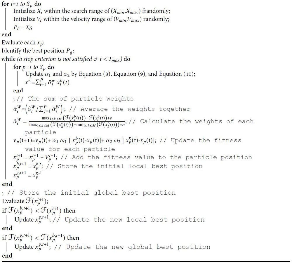$$ S_{p} $$, the maximum number of iteration $$ T_{max} $$.

4.2. Safety-aware IPSO multi-waypoint path planning

To ensure the robot safely reaches the waypoints via the planned visiting sequence, the safety-aware road is selected to guide the autonomous robot. Nevertheless, there is a problem with the connection path from the location of the waypoints to safety-aware roads. When we integrate the position information of a waypoint in the workspace, it may be necessary to obtain the collision-free connection path length from the waypoint to all nodes, which is computationally expensive. As shown in Figure 6A, with $$ \mathcal{N} $$ nodes obtained in the workspace, there are $$ \mathcal{N} $$ possible connection paths from the waypoints to the nodes in the workspace. With the initial $$ \mathcal{N} \times \mathcal{N} $$ adjacent distance matrix obtained from GVD graph and the increasing $$ \mathcal{M} $$ waypoints in the workspace, the size of new distance matrix is expanded to $$ (\mathcal{N}+\mathcal{M}) \times (\mathcal{N}+\mathcal{M}) $$. Since most of the connection path computations are unnecessary, a new adjacent node selection (ANS) algorithm is proposed to reduce the computational effort by restricting the search space in local regions rather than the entire working region.

The local regions are shown in Figure 6B, and the dark blue nodes, such as $$ \alpha $$ and $$ \beta $$ nodes in the regions, are potential adjacent nodes to connect. The radius $$ \mathcal{R} $$ of the local area shall be determined by the potential workspace, which determines the number of nodes in the search range. For instance, in an area with clustered obstacles, there are many nodes in the environment; thus, the search radius may be small. However, In an area with sparse obstacles, there are fewer nodes in the environment; thus, the search radius needs to be larger to include all potential nodes.

Since the entire workspace is projected through the GVD graph, we can interpret the sparseness of the entire workspace through the distance of the edge list $$ \mathcal{E} $$. Nevertheless, some edge distances cannot represent the sparseness of the entire workspace, such as the edges enclosed by the red dotted line in Figure 6B.

Therefore, to exclude these extraneous edges of distance, we sort the entire edge list before removing the lowest $$ 10\% $$. The radius $$ \mathcal{R} $$ of the search range is defined as the average of the remaining edge distance. After obtaining the nodes in the search environment, we plan a collision-free trajectory from the current waypoint to reach each node through the IPSO algorithm.

The IPSO navigation algorithm is initiated in the search range to obtain the optimal path. The local search region is interpreted into grid-based map, where the obstacle areas are inaccessible grids in the workspace. Dijkstra's algorithm is utilized as a local search algorithm and the cost function within the model. For graph-based maps, they must be a method for traveling from one node to another utilizing the edges within the graph. One method of this is Dijkstra's algorithm, which utilizes a weighted graph to determine the shortest path from a source node to a target node. The algorithm also keeps track of the known shortest distances from each node while simultaneously updating their weights to improve the overall shortest path from each node. By recursively establishing a path with random solutions generated in the workspace, the IPSO algorithm can construct the collision-free path with the least fitness value, which also represents the path with minimum length. Therefore, the length of the connecting path $$ \mathcal{L}_{c} $$ can be obtained, and by combining the length of the GVD path $$ \mathcal{L}_{e} $$, the optimal safety-aware trajectory is obtained as shown in Figure 6C.

To effectively reduce and smooth the overall path from each waypoint to the waypoint, various methods have been developed to achieve this goal, for example, the $$ \mathcal{B} $$-spline curve, which works by taking a set of points that are used to curve sharp close turns around obstacles and is very effective and thus widely used in smooth polylines, due to its closed-form expression of the position coordinates. The original methodology of the $$ \mathcal{B} $$-spline curve method, in some cases, changes the trajectory of the original path created by the global navigation system. The problem can be mediated by implementing the piecewise $$ \mathcal{B} $$-spline method, which only smooths the path around each obstacle. Lei et al. evaluated the effectiveness of the improved $$ \mathcal{B} $$-spline method, and ultimately found that the hybrid method was able to reduce the overall all path in point-to-point navigation ^[38]. The $$ \mathcal{B} $$-spline curve can be defined by a cardinal functions $$ L_{j, r}(q) $$, control points $$ B_{j} $$ and degree $$ (r - 1), $$ which is given by the following equations.

(11) $$ \begin{equation} \begin{array}{l} K(q)= \sum L_{j, r}(q) B_{j} \end{array} \end{equation} $$

where $$ B_{j} = [B_{jx}, B_{jy}] $$ are the $$ (n + 1) $$ control points and a knot vector $$ u $$. $$ N_{i, k}(u) $$ are the basic functions, which are defined recursively as follows:

(12) $$ \begin{equation} \begin{array}{l} L_{j, r}(q) = \frac{(q-x_{j})}{x_{j+r-1}-x_{j}} N_{j, r-1}(q) + \frac{(x_{j+r}-q)}{x_{j+r}-x_{j+1}} N_{j+1, r-1}(q) \end{array} \end{equation} $$

(13) $$ \begin{equation} L_{j, r}(q) = \begin{cases} 1, \; \; \; \; q_{j} q_{j}\le q \le q_{j+1}\\ 0, \; \; \; \; \; \;\; \; otherwise \end{cases} ; \; q \in [0, 1] \end{equation} $$

Geometric continuity $$ G^2 $$ is the metric used to evaluate smoothing methods, which is defined by the tangent unit and curvature vector at the intersection of two continuous segments ^[38] [Figure 7A]. To achieve $$ G^2 $$ continuity, the control points $$ B_{j} $$ of $$ \mathcal{B} $$-spline curve to the path point, $$ Y_{j} $$, is defined as

(14) $$ \begin{equation} \begin{array}{l} B_{1} = Y_{j} - (1 +v)s_{2}q_{j-1}\\ B_{2} = -s_{2}q_{j-1}\\ B_{3} = Y_{j}\\ B_{4} = Y_{j}+s_{2}q_{j}\\ B_{5} = Y_{j} +(1 +v)s_{2}q_{j-1} \end{array} \end{equation} $$

where $$ c $$ is smoothing length ratio $$ v= s_{1}/s_{2} $$, and $$ q_{j-1} $$ defines the unit vector of $$ Y_{j-1}Y_{j} $$. $$ q_{j} $$ represents the unit vector of the line $$ Y_{j}Y_{j+1} $$. The combined sum of $$ s_{1} $$ and $$ s_{2} $$ is the smoothed length. The half of the corner angle is denoted as: $$ \Gamma = \beta / 2 $$. Using a knot vector of [0, 0, 0, 0, 0.5, 1, 1, 1, 1], the smoothing error distance $$ \epsilon $$ and maximum curvature $$ K_{max} $$ within the smooth path can be expressed as:

(15) $$ \begin{equation} \begin{array}{l} \epsilon = \frac{s_{2}\sin{\Gamma}}{2} \end{array} \end{equation} $$

(16) $$ \begin{equation} \begin{array}{l} R_{max} = \frac{4\sin{\Gamma}}{3s_{2}\cos^2{\Gamma}} \end{array} \end{equation} $$

Using the previous equations the smoothing error distance $$ \epsilon $$ can be defined by the existing maximum curvature $$ R_{max} $$ given by the robot:

(17) $$ \begin{equation} \begin{array}{l} \epsilon = \frac{2\tan^2{\Gamma}}{3R_{max}} \end{array} \end{equation} $$

The improved $$\mathcal{B}$$-spline model has specific advantages over the basic $$\mathcal{B}$$-spline model, one of which is its ability to smooth many different trajectories with various angles, as seen in Figure 7B. The curve produced by the improved $$\mathcal{B}$$-spline model is significantly closer to the original path than the original model. When considering the constraints of the robot, the improved $$\mathcal{B}$$-spline mode performs {better} in various degrees of angles. The overall advantages of the improved $$\mathcal{B}$$-spline model are as follows:

(1) The path generated is tangent and curvature continuity, so that the robot can have a smooth steering command, which can correct any discontinuity of normal acceleration and establish a safer path for the robot to follow.

(2) The improved model generates a better curve by solely affecting the two lines within the corner of the original trajectory. Each curve generated affects others within the lines.

(3) The improved model easily adjusts to the smoothed path based on the environment constraints or the robot.

Algorithm 2: Pseudocode for the adjacent node selection (ANS) algorithm

Input: Edge list $$ \mathcal{E} $$, $$ \mathcal{N} $$ nodes coordinates ($$ \mathbb{N}_x, \mathbb{N}_y $$), $$ \mathcal{N} \times \mathcal{N} $$ distance matrix $$ \mathcal{D} $$ and the location of the waypoint $$ \alpha $$, ($$ \alpha_x, \alpha_y $$) and the waypoint $$ \beta $$, ($$ \beta_x, \beta_y $$).

Output: The path length of the trajectory 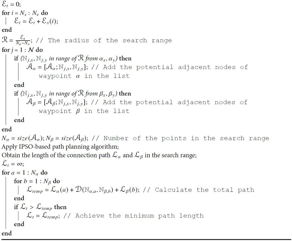$$ \mathcal{L}_{t} $$

$$ N_e = size(\mathcal{E}) $$; // Number of the edges in the workspace

$$ [\mathcal{E}_s, sortInd]=sort(\mathcal{E}) $$; // Sort the edge list from low to high

$$ N_s = \lceil \frac{N_e}{10} \rceil $$; // Exclude 10% of extraneous edge distance

5. REACTIVE LOCAL NAVIGATION

A crucial aspect in developing a multi-waypoint model is accounting for moving and unknown obstacles ^{[39, 40]}. In a real-world setting, not all objects are static and known. To develop a more efficient model, we propose the use of a local navigator to remedy this issue.

In order to avoid dynamic and unknown obstacles, the proposed model employs the Vector Field Histogram (VFH) model as a reactive local navigator. An autonomous robot uses a velocity command to and from each waypoint, provided by the local navigator ^[41]. By applying the VFH to the overall global trajectory with a sequence of markers, the path can be broken down into various segments to improve the efficiency in obstacle-populated workspaces. The local navigator builds a map depicting the free space and obstacles in the map by utilizing a 2D histogram grid with equally sized cells ^[42]. As the robot follows the generated trajectory within the workspace, the map is simultaneously built, shown in Figure 8. In developing an autonomous obstacle avoidance model, concurrent map building and navigation are crucial. The robot pose $$ (X, Y, Yaw) $$ is used to determine the map building. Thus, the precise registration of the built local map as a part of the global map can

be carried out. This map building aims to construct an occupancy-cell-based map. The values for each cell in the map vary over the range [-127, 128] ^[42]. The initial value is zero, which indicates that the cell is neither occupied nor unoccupied. The value is 128 if one cell is occupied with certainty and -127 if one cell is unoccupied with certainty. The values falling into (-127, 128) express contain a level of certainty in the range. When the VFH model is employed in conjunction with the GVD and IPSO algorithm, the robot can be successfully navigated through our built map with obstacle avoidance. In combination with our local navigator, a sensor configuration can be developed for the local navigator to perform it. In Figure 9 one can see the overview of our sensor configuration. The proposed configuration utilizes a 270-degree SICK LMS LiDAR sensor to detect obstacles within a range of 20 m @ 0.25-degree resolution. The LiDAR sensor scans at a rate of 25Hz. Then, it needs a method of finding our current position and the waypoints within the map. A Novatel's ProPak-LB Plus DGPS sensor is utilized to obtain our current position and how it correlates to the coordinates of each waypoint. Next, a PNI TCM6 digital compass is employed to establish our heading with an accuracy of 0.5 degrees. The sensor updates at 20Hz, which allows the robot to operate efficiently. Lastly, the configuration utilizes an AVT Stingray F-080C 1/3" CCD camera, which enables our robot to sense obstacles of various heights, shapes and sizes. The stingray camera is perfect for robot vision because it uses the IIDC IEEE 1394B protocol to transfer images. The system needs a computer system to house our operating system, sensor data, and programs for the robot. In this portion of the sensor configuration, a MackBook Pro i s equipped to suit our needs. The last step in the process is to establish a method of communication from the sensors to the computer systems. A sort of UART to USB hub is utilized for this purpose and fuses the sensor data together without losing any sensor information. The type of sensor confusion can be used on most ground-based robot systems for indoor and outdoor use.

6. SIMULATION AND COMPARISON STUDIES

In this section, simulation and comparison studies are performed to illustrate the value and vitality of the proposed model. In the first experiment, simulations are conducted using a well-known Traveling Salesman Problem (TSP) based data set, and results are compared with other heuristic-based algorithms. The proposed model is thoroughly evaluated in the second experiment through a comparison study using a similar model proven to work effectively for multi-waypoint navigation.

6.2. Model comparison studies

The compared models were developed to address the issues of multi-waypoint navigation and mapping in various applications. Each model uses some variation of a global navigation system in combination with an obstacle avoidance technique. The models were selected based on their map configuration and overall efficiency in solving the multi-waypoint navigation problem. Our comparison studies analyze the number of nodes, the trajectories produced, and the total time to fulfill the fastest route.

It is clear that the waypoint order and paths obtained by each model are created in an obstacle-free environment, as illustrated in Figure 10A. The length created by the Zhang's model was 240.84 m, while the proposed model produced a shorter trajectory of 219.99 m. This is due to the founded waypoint orders in the environment. In Zhang's comparison study, the proposed model establishes more nodes, and the overall path is expanded by 1.09%, but the proposed model generates a solution 6.1% faster than the compared model. Zhang's proposed model has to utilize a node selection algorithm to establish its shortest path, while the proposed model does not. Due to this feature, the compared model was evaluated before this crucial step and discovered that the nodes established were vastly greater than the proposed model, as seen in Table 2. Considering this factor, the proposed model can surpass and outperform Zhang's model. Asl and Taghirad aimed to solve the multi-goal navigation problem by developing a traveling salesman problem in the belief space ^[44].

Table 2

An illustration of the number of nodes, distance, and time spent traversing with the map to each waypoint

Model	Nodes	Distance	Time spent s
Zhang's model before node reduction	242	271.1	2.25
Zhang's model after node reduction	24	253.4	0.66
Proposed model	38	277.7	0.40

From Figure 11, one can see the established path using both Asl's method as well as the method proposed in this paper. The method proposed by Asl and Taghirad has the advantage of creating a shorter path but requires a greater number of nodes than the proposed method. Figure 12 depicts the model comparison between Zhuang et al.'s model and the proposed method^[45]. The simulation studies reveal that the proposed model had an increased length of approximately 0.05% over Zhuang et al.'s model. Once the compared model requires a greater number of nodes to complete its multi-waypoint navigation, another key point from this comparison is the path created from Zhuang et al.'s model and the proximity to the obstacles in the map. In a real-world environment, the robot could obtain server damage or cause an accident if it is too close to the surrounding obstacles^[45]. The proposed method established an effective path without risking the robots well being. Von{á}sek and P{e}ni{c}ka ^[46] models had similar results to the previous models, with an increased length of approximately 0.05%, as seen in Figure 13. The two compared models have the same problem as Zhuang et al.' model^[45]. The paths are excessively close to obstacles in the map and thus are not efficient for real-world implementation.

In such an environment, it is very important to consider the robot safety because of the narrow paths created being tightly packed with triangular shaped obstacles. Although most of our model comparison results showed that the path constructed with the proposed model increased from the compared models, we achieved our goal of constructing safety-aware roads for robot safety and establishing an obstacle-free path.

From Figure 14, it is observed how the local navigator establishes a map through vision sensors such as LiDAR. In Figure 14, it is obvious that the map in various stages is shown as the robot traverses along the generated trajectory found in the Vonásek's simulation [Figure 13]^[46].

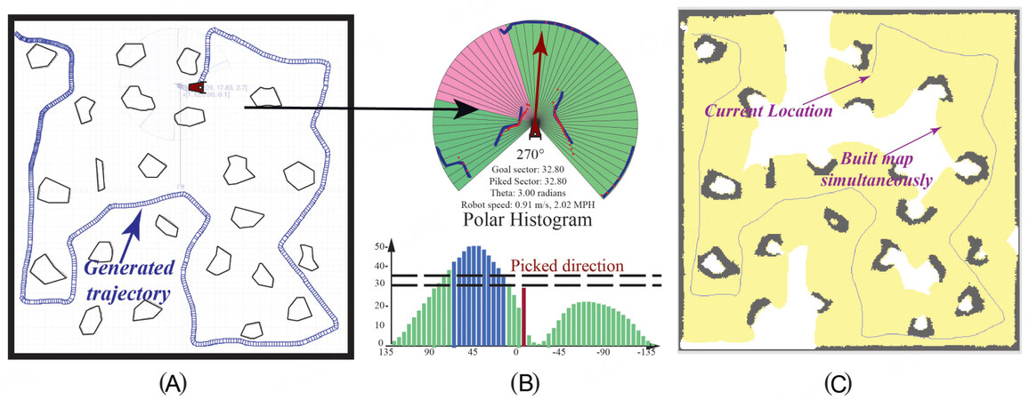
Figure 14. Illustration of the scenario in Figure 13 navigation and mapping simulation. (A) It depicts the robot traversing a majority of the map, while avoiding obstacles in the environment. (B) It illustrates a polar histogram and how the obstacles are viewed while the robot is in motion, as well as points of high impact. The obstacles are viewed as lines since the LiDAR sensor can only see the part of the object that faces the LiDAR sensor. The picked direction portion of part (B) depicts the probability of colliding with obstacles while also selecting the best direction to move the robot. (C) It demonstrates the map being simultaneously built as the the robot traverses the established trajectory.

The robot is able to reconstruct the outer boundary of the obstacles through the LiDAR scan. These are depicted as the poly-shaped figures with a rough background and a white center.

In Figure 15A, it is clear to see the original starting position as well as the planned trajectory, which was found utilizing our proposed IPSO model. From the figures, one could observe fully and partly detected obstacles as well as the outer boundary being detected. The map depicted in Figure 15 has a height and width of 60 $$ m $$. The dimensions of the robot are approximately 0.82 $$ m $$ long and 0.68 $$ m $$ wide. In Figure 15A, the robot has successfully traversed one third of the map, while simultaneously avoiding the obstacles. In Figure 15B, it illustrates the robot's planned trajectory and the map being simultaneously constructed along the path. The portions of the figure depicted in a yellow field are the built map sensed by the onboard sensors. Finally, in Figure 15C, the robot has successfully visited each waypoint and reached its final destination, and it shows the complete depiction of the map along the projected path.

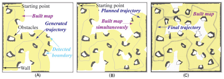
Figure 15. Illustration of the navigation and mapping ability of the proposed model. (A) The robot follows the generated trajectory and detects obstacle boundaries by the LiDAR sensor. (B) The simultaneous map building and navigation capabilities of the proposed model. (C) The fully generated trajectory and established map.

7. CONCLUSION

We proposed an adjacent node selection (ANS) algorithm to find a node in the graph to connect waypoints. This algorithm is utilized in the safety-aware multi-waypoint navigation and mapping by an improved PSO and GVD model.An IPSO-based multi-waypoint algorithm has been developed to define an order for waypoint navigation. Through our proposed ANS algorithm, connections among the waypoints and the safety-aware routes to reach multi-objective optimization can be created. The feasibility and effectiveness of our model by conducting a benchmark test and model comparison studies and analyses have been demonstrated.

DECLARATIONS

REFERENCES

1. Chu Z, Wang F, Lei T, Luo C. Path planning based on deep reinforcement learning for autonomous underwater vehicles under ocean current disturbance. IEEE Trans Intell Veh 2022:1-1.
2. Zhao W, Lun R, Gordon C, et al. A privacy-aware Kinect-based system for healthcare professionals. In: IEEE International Conference on Electro Information Technology. Grand Forks, USA; 2016. pp. 205-10.
3. Zhao W, Lun R, Gordon C, et al. Liftingdoneright: a privacy-aware human motion tracking system for healthcare professionals. Int J Handheld Comput Res 2016;7:1-15.
4. Lei T, Luo C, Jan GE, Bi Z. Deep learning-based complete coverage path planning with re-joint and obstacle fusion paradigm. Front Robot AI 2022;9.
5. Li X, Luo C, Xu Y, Li P. A Fuzzy PID controller applied in AGV control system. In: International Conference on Advanced Robotics and Mechatronics. Macau, China; 2016. pp. 555-60.
6. Lei T, Luo C, Ball JE, Bi Z. A hybrid fireworks algorithm to navigation and mapping. In: Handbook of Research on Fireworks Algorithms and Swarm Intelligence. IGI Global; 2020. pp. 213-32.
7. Jayaraman E, Lei T, Rahimi S, Cheng S, Luo C. Immune system algorithms to environmental exploration of robot navigation and mapping. In: International Conference on Swarm Intelligence. Qindao, China: Springer; 2021. pp. 73-84.
8. Yang J, Chai T, Luo C, Yu W. Intelligent demand forecasting of smelting process using data-driven and mechanism model. IEEE Trans Ind Electron 2018;66:9745-55.
9. Zhu D, Tian C, Jiang X, Luo C. Multi-AUVs cooperative complete coverage path planning based on GBNN algorithm. In: Chinese Control and Decision Conference. Chongqing, China; 2017. pp. 6761-66.
10. Luo C, Yang SX, Mo H, Li X. Safety aware robot coverage motion planning with virtual-obstacle-based navigation. In: IEEE International Conference on Information and Automation. Lijiang, China; 2015. pp. 2110-15.
11. Wang L, Luo C. A hybrid genetic tabu search algorithm for mobile robot to solve AS/RS path planning. Int J Rob Autom 2018;33:161-68.
12. Wang L, Luo C, Cai J. A variable interval rescheduling strategy for dynamic flexible job shop scheduling problem by improved genetic algorithm. J Adv Transp 2017;2017.
13. Qu Q, Zhang H, Luo C, Yu R. Robust control design for multi-player nonlinear systems with input disturbances via adaptive dynamic programming. Neurocomputing 2019;334:1-10.
14. Penicka R, Scaramuzza D. Minimum-time quadrotor waypoint flight in cluttered environments. IEEE Rob Autom Lett 2022;7:5719-26.
15. Jan GE, Luo C, Lin HT, Fung K. Complete area coverage path-planning with arbitrary shape obstacles. J Autom Contr Eng 2019;7.
16. Lei T, Sellers T, Rahimi S, Cheng S, Luo C. A nature-inspired algorithm to adaptively safe navigation of a Covid-19 disinfection robot. In: International Conference on Intelligent Robotics and Applications. Cham: Springer; 2021. pp. 123-34.
17. Lei T, Luo C, Sellers T, Wang Y, Liu L. Multi-task allocation framework with spatial dislocation collision avoidance for multiple aerial robots. IEEE Trans Aerosp Electron Syst 2022; doi: 10.1109/TAES.2022.3167652.
18. Chen Y, Liu C, Shi BE, Liu M. Robot navigation in crowds by graph convolutional networks with attention learned from human gaze. IEEE Rob Autom Lett 2020;5:2754-61.
19. Chen J, Luo C, Krishnan M, Paulik M, Tang Y. An enhanced dynamic Delaunay triangulation-based path planning algorithm for autonomous mobile robot navigation. In: Intelligent Robots and Computer Vision XXVⅡ: Algorithms and Techniques. vol. 7539. California, USA: SPIE; 2010. pp. 253-64.
20. Luo C, Xiao Y, Yang SX, Jan GE. Improving vehicle navigation by a heading-enabled ACO approach. In: World Automation Congress. Rio Grande, USA: IEEE; 2016. pp. 1-6.
21. Lei T, Luo C, Jan GE, Fung K. Variable speed robot navigation by an ACO approach. In: International Conference on Swarm Intelligence. Cham: Springer; 2019. pp. 232-42.
22. Wang L, Luo C, Li M, Cai J. Trajectory planning of an autonomous mobile robot by evolving ant colony system. Int J Rob Autom 2017;32:406-13.
23. Lei T, Luo C, Sellers T, Rahimi S. A bat-pigeon algorithm to crack detection-enabled autonomous vehicle navigation and mapping. Intell Syst Appl 2021;12:200053.
24. Luo C, Yang SX, Krishnan M, Paulik M. An effective vector-driven biologically-motivated neural network algorithm to real-time autonomous robot navigation. In: IEEE International Conference on Robotics and Automation. Hong Kong, China; 2014. pp. 4094-99.
25. Na YK, Oh SY. Hybrid control for autonomous mobile robot navigation using neural network based behavior modules and environment classification. Auton 2003;15:193-206.
26. Zhong C, Luo C, Chu Z, Gan W. A continuous hopfield neural network based on dynamic step for the traveling salesman problem. In: International Joint Conference on Neural Network. Anchorage, USA: IEEE; 2017. pp. 3318-23.
27. Lazreg M, Benamrane N. Hybrid system for optimizing the robot mobile navigation using ANFIS and PSO. Rob Auton Syst 2022;153:104114.
28. Jensen-Nau KR, Hermans T, Leang KK. Near-optimal area-coverage path planning of energy-constrained aerial robots with application in autonomous environmental monitoring. IEEE Trans Autom Sci Eng 2021;18:1453-68.
29. Janoš J, Vonásek V, Pěnička R. Multi-goal path planning using multiple random trees. IEEE Rob Autom Lett 2021;6:4201-8.
30. Ortiz S, Yu W. Autonomous navigation in unknown environment using sliding mode SLAM and genetic algorithm. Intell Robot ;1:131-50.
31. Bernardo R, Sousa J, Gonçalves PJ. Planning robotic agent actions using semantic knowledge for a home environment. Intell Robot 2021;1:101-15.
32. Luo C, Yang SX. A bioinspired neural network for real-time concurrent map building and complete coverage robot navigation in unknown environments. IEEE Trans Neural Netw 2008;19:1279-98.
33. Shair S, Chandler JH, GonzÁlez-Villela VJ, Parkin RM, Jackson MR. The use of aerial images and GPS for mobile robot waypoint navigation. IEEE/ASME Trans Mechatron 2008;13:692-99.
34. Yang Y, Khalife J, Morales JJ, Kassas ZM. UAV waypoint opportunistic navigation in GNSS-denied environments. IEEE Trans Aerosp Electron Syst 2022;58:663-78.
35. Teng F, Zhang H, Luo C, Shan Q. Delay tolerant containment control for second-order multi-agent systems based on communication topology design. Neurocomputing 2020;380:11-19.
36. Lee DT, Drysdale RL ó. Generalization of Voronoi diagrams in the plane. SIAM J Comput 1981;10:73-87.
37. Takahashi O, Schilling RJ. Motion planning in a plane using generalized Voronoi diagrams. IEEE Trans Robot 1989;5:143-50.
38. Lei T, Luo C, Ball JE, Rahimi S. A graph-based ant-like approach to optimal path planning. In: IEEE Congress on Evolutionary Computation. Glasgow, UK; 2020. pp. 1-6.
39. Li X, Li X, Khyam MO, Luo C, Tan Y. Visual navigation method for indoor mobile robot based on extended BoW model. CAAI Trans Intell Tech 2017;2: 142-47. Available from: https://ietresearch.onlinelibrary.wiley.com/doi/full/10.1049/trit.2017.0020[Last accessed on 31 Aug 2022].
40. Yang Y, Deng Q, Shen F, Zhao J, Luo C. A shapelet learning method for time series classification. In: IEEE International Conference on Tools with Artificial Intelligence. San Jose, USA; 2016. pp. 423-30.
41. Liu L, Luo C, Shen F. Multi-agent formation control with target tracking and navigation. In: IEEE International Conference on Information and Automation. Macao, China; 2017. pp. 98-103.
42. Babinec A, Duchoň F, Dekan M, Pásztó P, Kelemen M. VFH*TDT (VFH* with time dependent tree): A new laser rangefinder based obstacle avoidance method designed for environment with non-static obstacles. Rob Auton Syst 2014;62:1098-115.
43. Zhang B, Jin W, Gao X, Chen W. A multi-goal global dynamic path planning method for indoor mobile robot. In: International Symposium on Robotics Intelligent Manufacturing Technology. Changzhou, China; 2021. pp. 97-103.
44. Noormohammadi-Asl A, Taghirad HD. Multi-goal motion planning using traveling salesman problem in belief space. Inf Sci 2019;471:164-84.
45. Zhuang H, Dong K, Qi Y, Wang N, Dong L. Multi-destination path planning method research of mobile robots based on goal of passing through the fewest obstacles. Appl Sci 2021;11:7378.
Cite This Article
Export citation file: BibTeX | RIS
OAE Style
Sellers T, Lei T, Luo C, Eu Jan G, Ma J. A node selection algorithm to graph-based multi-waypoint optimization navigation and mapping. Intell Robot 2022;2(4):333-54. http://dx.doi.org/10.20517/ir.2022.21
AMA Style
Sellers T, Lei T, Luo C, Eu Jan G, Ma J. A node selection algorithm to graph-based multi-waypoint optimization navigation and mapping. Intelligence & Robotics. 2022; 2(4): 333-54. http://dx.doi.org/10.20517/ir.2022.21
Chicago/Turabian Style
Sellers, Timothy, Tingjun Lei, Chaomin Luo, Gene Eu Jan, Junfeng Ma. 2022. "A node selection algorithm to graph-based multi-waypoint optimization navigation and mapping" Intelligence & Robotics. 2, no.4: 333-54. http://dx.doi.org/10.20517/ir.2022.21
ACS Style
Sellers, T.; Lei T.; Luo C.; Eu Jan G.; Ma J. A node selection algorithm to graph-based multi-waypoint optimization navigation and mapping. Intell. Robot. 2022, 2, 333-54. http://dx.doi.org/10.20517/ir.2022.21
About This Article
Copyright
Data & Comments
Data
Cite This Article 27 clicks
Like This Article 0
likes
Comments
Comments must be written in English. Spam, offensive content, impersonation, and private information will not be permitted. If any comment is reported and identified as inappropriate content by OAE staff, the comment will be removed without notice. If you have any queries or need any help, please contact us at support@oaepublish.com.