
An overview of intelligent image segmentation using active contour models


Abstract
The active contour model (ACM) approach in image segmentation is regarded as a research hotspot in the area of computer vision, which is widely applied in different kinds of applications in practice, such as medical image processing. The essence of ACM is to make use ofuse an enclosed and smooth curve to signify the target boundary, which is usually accomplished by minimizing the associated energy function by means ofthrough the standard descent method. This paper presents an overview of ACMs for handling image segmentation problems in various fields. It begins with an introduction briefly reviewing different ACMs with their pros and cons. Then, some basic knowledge in of the theory of ACMs is explained, and several popular ACMs in terms of three categories, including region-based ACMs, edge-based ACMs, and hybrid ACMs, are detailedly reviewed with their advantages and disadvantages. After that, twelve ACMs are chosen from the literature to conduct three sets of segmentation experiments to segment different kinds of images, and compare the segmentation efficiency and accuracy with different methods. Next, two deep learning-based algorithms are implemented to segment different types of images to compare segmentation results with several ACMs. Experimental results confirm some useful conclusions about their sharing strengths and weaknesses. Lastly, this paper points out some promising research directions that need to be further studied in the future.
Keywords
1. INTRODUCTION
Image segmentation is a significant component in image processing, and serves as the foundation for image analysis and image understanding. The accuracy of image segmentation hugely affects the quality of subsequent image processing procedures. Its major role is to separate the input images into a series of disjoint sub-regions with unique features, and extract objects of interest. Therefore, image segmentation has been extensively employed in a variety of areas such as medical image processing [1-4], target recognition [5-8], moving target tracking [9-12], etc.
In the last decade, active contour model (ACM) using the level set approach has become one of the most efficient tools for image segmentation, which has been extensively employed in tasks of image segmentation. The image segmentation algorithm based on ACM is an image processing technique that combines upper-level and various prior knowledge for stable image segmentation, which can add image grayscale and edge information during the process of optimization. It provides a piece-wise smooth closed contour as the final outcome, which haswith superior performance such as diverse forms and flexible structures. ACM converts the image segmentation problem into the process of solving a minimization problem with the energy function. The contour of the target object is expressed by means of the zero level set in the execution process, which is convenient to dealfor dealing with the topological deformation during the curve evolution. Nevertheless, the topology of the segmented region changes in an automatic and uncontrollable manner can either be an advantage or an inconvenience according to different applications. The essence of ACM is to employ a continuous and closed curve to represent object boundary, which is achieved through the standard gradient descent approach to minimize the associated energy function.
ACMs are generally comprised of two categories: parametric ACMs and geometric ACMs. In parametric ACMs [13,14], the evolution curve is described in the parametric form to obtain object boundary. However, parametric ACMs can only deal with images that include a sole target object with an obvious boundary through the process of parameterization. Most importantly, they cannot automatically handle topology changes during the process of curve evolution. The geometric ACM is also named as the level set method, which guides evolution curves to evolve towards the target boundary through the geometric measurement parameters. The introduction of level set methods makes it possible to segment images with multiple target objects simultaneously, and solves the issue of topology changes (merging or broken curves) caused by the process of parameterization in parametric ACMs. This paper mainly pays attention to the existing geometric ACMs, and they can be further categorized into three types: region-based ACMs [15-17], which aim at identifying each region of interest using a defined region descriptor to guide the evolution motion of active contour; edge-based ACMs [18,19], which utilize gradient information of the target boundary as the major driving force to attract the active contour to the object boundary; and hybrid ACMs [20-24], which combine local region and edge information together to instruct evolution curve to move towards target boundary.
The Chan-Vese (CV) model [15] utilized the average gray values of the outside and inside areas of the contour to characterize the foreground and background of the input image, respectively. As a classical region-based ACM, CV model does not need to utilize image gradient information, which makes it very suitable to segmentfor segmenting images with blurred or discontinuous edges. However, for images with uneven grayscale such as images subjected to uneven illumination, CV model could obtain undesired segmentation results in the form of having difficulty extracting meaningful objects out of images and falling into local minima [25]. To solve this issue, the pieceiwse piecewise smooth (PS) model [26] was developed to segment images with intensity non-uniformity to some degree due to the consideration of image local attributes. Nevertheless, PS model is sensitive to different initial contours and inefficient due to the complex computation process. The geometric active contours (GAC) model [27,28] translated curve evolution into the evolution of level set function through variational methods, which effectively solves topology change problems. However, this model has to continuously re-initialize the level set function to zero level set, which results in inefficient segmentation and possible boundary leakage. In addition, the segmentation results of medical images that usually contain noise and blurred or discontinuous edges are poor. The fast global minimization (FGM) model [29] defined global minimizers to overcome the drawback of falling into local minima in the local optimization approach such as CV model [15], which enables the FGM model to be independent of random positions of initial contours and gets rid of frequent re-initialization of distance function in GAC model [28]. The model [30] was competent to obtain the global minimum of an ACM between two sides, which enables the initialization process easier and reduces the chance of falling into a local minimum at the false edge. The key of this model is to take advantage of a novel numerical method to compute the minimum route, which is the global minimum of the associated energy function among all routes connecting the two end points.
To make the level set function inherently stable, the distance regularized level set evolution (DRLSE) model [31] added a distance regularization term, which controls the deviation between the level set function and the standard signed distance function during the curve evolution. In addition, this model avoided the problem of constant re-initialization during the curve evolution. Nevertheless, this model has no self-adjustment ability during the process of energy minimization due to uni-directional area term, and remains sensitive to different selections of initial contours. The bias correction (BC) model [32] was designed to segment the image and compute the bias field simultaneously to correct unevenly distributed intensity in medical images, which is more precise and has less segmentation time than the famous PS model. However, this model is nowadays inefficient and less accurate than many newly developed ACMs. In addition, it is not very effective in segmenting natural images taken from nature. The local binary fitting (LBF) [33] and region- scalable fitting (RSF) [34] models were constructed to segment images with intensity non-uniformity, which use a kernel function to design a local binary fitting energy and embeds information of local area to guide the motion of level set function. In addition, these two models incorporates a penalty term in the energy function, which avoids the periodic re-initialization process and greatly improves algorithm efficiency. However, the introduced kernel function only calculates the grayscale value of image locally, which makes it possible to get trapped into local minimum during the procedure of minimizing its energy. In other words, these two models are sensitive to initial contours. In addition, it takes time to calculate the two fitting functions that need to be continuously updated during each iteration, resulting in the inefficient segmentation of RSF model. The local image fit (LIF) model [35] considered the technique of Gaussian filtering and local image information to segment different images with intensity non-uniformity, which segments images faster than RSF model due to only two convolution operations during each iteration. However, this model still remains susceptible to different initial contours. Specifically, an inappropriate initial contour may result in a wrong segmentation due to the fact that the majority of existing ACMs have non-convex energy functions. To solve the issue of non-convex functions, the approach [36] was designed to translate non-convex function to convex function, which handles the problem of local minima frequently occurred occurring in non-convex function. Nevertheless, this approach is too complex and time-consuming to be applied in practice. In addition, the method [37] numerically tracked an accurate numerical approximation of the most optimized solution for some relaxed problems, which is capable of providing a close bound between the calculated solution and the real minimizer. Nevertheless, this model is not guaranteed to obtain a global minimizer of the minimal partition problem (also known as spatially continuous Potts model).
The local and global intensity fitting (LGIF) model [38] was defined as a linear combination of local image fit (LIF) energy and global image fit (GIF) energy. By choosing the appropriate weights that are used to control the ratio of LIF energy and GIF energy, this model can effectively handle the grayscale non-uniformity and has good initialization robustness. However, the weights of LIF and GIF models are unpredictable for different images and often need to be manually calibrated with respect to the degree of grayscale non-uniformity. The segmentation will fail if it is chosen poorly [39]. The local gaussian distribution fitting (LGDF) model [40] defined a fitting energy based on the mean and variance of the local gray values. Compared with RSF model, this model is able to segment local areas with the same mean gray value but different variances. However, this model is less efficient than RSF model due to the fact that more time is consumed to compute the variances. In addition, this model is also sensitive to different initial contours [41].
The core of local region Chan-Vese (LRCV) model [42] was to replace two fitting constants in the CV model with the two fitting functions in RSF model. In addition, this model utilizes the segmentation result of degraded CV model as the initial contour, which can reduce the dependence on the initial contour to a certain extent and accelerate the segmentation speed at the same time. Considering that many targets and backgrounds in real images are random, the local histogram fitting (LHF) model [43] took the advantage of two fitted histograms to approximate the distribution of the target and background, which can be used to segment regions with unpredictable distributions. However, it is inefficient because it needs to calculate the histogram distribution for each gray level (0-255). Similarly, it is sensitive to the initial contours. The local and global Gaussian distribution fitting (LGGDF) model [44] constructed a linear combination of a local and global Gaussian fit energies with a changeable weight to balance the local and global energies, which further decreases the dependence on the choices of initial contours. However, it is computationally intensive and the adaptive weight does not work well for some images. The local likelihood image fitting (LLIF) model [45] mainly utilized mean intensity and variance information of the local region. In fact, LLIF model is a combination of LIF model and LGDF model, which has enhanced applicability for segmenting images. However, the segmentation efficiency is relatively low, while the robustness to initialization is not appealing [46].
The RSF&LoG model [39] combined RSF model with optimized Laplacian of Gaussian (LoG) energy to improve segmentation results, which further improve sensitivity to different initial contours. Nevertheless, the segmentation time of this model is relatively long [47] due to the unoptimized computation procedure. The local pre-fitting (LPF) model [48] pre-calculated mean intensities of local regions ahead of iteration to obtain faster segmentation speed. Nevertheless, this model still faces some common issues such as stagnation of false boundaries, under- segmentation [49]. Therefore, the segmentation accuracy of this model still has space to be further improved. The LPF & FCM model [41] locally fitted out two fuzzy center points inside and outside the evolution curve ahead of iteration through the fuzzy c-means (FCM) clustering algorithm, which reduces computation cost and improves segmentation efficiency. In addition, this model puts combines an adaptive edge indicator function and an adaptive sign function together to resolve the issue of single direction of evolution contour to realize bidirectional motion.
The super-pixel based via a local similarity factor and saliency (SLSFS) model [50] linked super-pixel with FCM clustering algorithm to create initial contours, which is competent to create adaptive initial contour in the neighborhood of the target and effectively protect weak edge information. The model [51] constructed an adaptive weight ratio to calibrate the relationship between local energy part and global energy part, which is capable of automatically calibrating the direction of curve evolution with respect to the location of the target region. Nevertheless, the initial contour still has to be manually labeled during the process of curve evolution. The approach [52] associated the level set method (LSE) model [32] with region and edge synergetic level set framework (RESLS) model [53] to improve segmentation results, which is able to efficiently segment images with unevenly distributed intensity and extends the two-phase model to multi-phase model. However, this model is sensitive to the choice of parameters and incompetent to in effectively processing natural images with complicated background information. The method [54] employed self- organizing maps (SOM) to cluster the input image into two regions: foreground and background regions, which decreases the interference of noise and enhances system robustness. However, compared with K-mean clustering algorithm, SOM algorithm may obtains relatively smaller lower computation precision owing to the update of neighborhood nodes. The global and local fuzzy image fitting (GLFIF) model [55] utilized a combination of global and local fitting energy to process images with noise and non-uniform intensity, which hugely decreases the influences of background noise and intensity non-uniformity to obtain accurate segmentation result.
The additive bias correction (ABC) model [56] employed the theory of bias field correction to effectively segment images with unevenly distributed intensity and achieved good segmentation results. However, the issue of under- segmentation may occur while segmenting images with Gaussian noise interference, as described in Section 4, which means that the anti-noise robustness of this model still has space to be optimized. The pre-fitting energy (PFE) model [47] calculated median intensities of local regions before iteration begins began to decrease segmentation time. In addition, this model contains a novel single well potential function and its corresponding evolution speed function to facilitate the evolution speed of the level set function to achieve fast image segmentation. However, issues of stagnation of false boundaries and under- segmentation may take placeoccur during the process of evolution process. The above said issues are illustrated and explained in detail in Section
In the beginning of this paper, the authors have briefly reviewed the diverse ACMs (region-based ACMs, edge-based ACMs, and hybrid ACMs) in the area of image segmentation with their pros and cons. Then, several typical models in region-based ACMs, edge-based ACMs, and hybrid ACMs have beenwere reviewed with their advantages and disadvantages, respectively. After that,
2. RELATED KNOWLEDGE
2.1. Curve evolution
Geometric ACMs [59-62] are mainly on the basis of partial differential equations (PDEs) and variational method, whose essence is to continuously evolve toward the direction of energy minimum under the constraint of image information and give conditions. The segmentation process is generally as follows: a closed curve is initialized on the given image. Then, the curve evolves under the combined effect of internal and external energies, and stops evolving when the energy function achieves a minimal value through gradient descent method. Lastly, the zero level set coincides with the target edge to complete segmentation.
The goal of the level set approach is to find out the zero level set, which represents the target boundary as energy function is minimized through standard descent method. In other words, this level set method utilizes zero level set one dimension higher to express the evolution result of low-dimensional target. During the curve evolution, the points on the curve move towards their normal directions at a certain velocity respectively, with time as a variable respectively according to a certain velocity. In addition, the speed and direction of the motion are mainly controlled by two parameters: curvature and unit normal vector.
A closed and smooth curve
where
where
Therefore, Equation (2) can be simplified as
where
2.2. Level set function
The fundamental idea of level set method is to express the evolution of a closed curve
The level set function is always a valid function when the topology of the closed curve or surface embedded in the level set function changes. Instead of tracking the position of the evolved curve, the level set function is continuously updated under the action of solving a partial differential evolution equation to figure out its zero level set when image segmentation is performed by the level set method. The zero level set at that moment is derived when the evolution process stops under some certain criteria, which means the position of the zero level set is the location of the object contour after segmentation.
2.3. Energy function
The internal energy is determined by the internal properties of the curve, which defines an enlargeable and bendable curve deformation energy term, and maintains the continuity and smoothness of the contour curve by adjusting the weights to control the consistency of the elastic tensor of curve bending and the rigid tensor of stretching. The external energy determined by image information consists of image constraint energy term and image potential energy term [65]. There is no fixed expression formula for the constraint energy term, which is usually constructed according to users' demands or image features. The external energy determines the evolution direction of the active contour, which guides the evolution contour line to evolve towards the target boundary.
3. ACTIVE CONTOUR MODEL
In this section, some representative ACMs in of three types (region-based ACMs, edge-based ACMs, and hybrid ACMs) are reviewed with their pros and cons in detail.
3.1. Region-based ACMs
3.1.1. Mumford Shah model
MS model [26] unifies image data, initial estimation and target contour in a feature extraction process under the constraint of knowledge, which is capable of autonomously converging to the energy minimum energy state after proper initialization. This model converts image segmentation issue into minimization of the energy function as follows:
where
The energy function in Equation (4) is comprised of three terms: the first data fidelity term (
3.1.2. Chan Vese model
CV model [15] considers the image global characteristics and image statistical information inside and outside the evolution curve to drive the curve to approach the contour of the target area, which achieves success in the segmentation of images with blurred edges and small gradient changes and remains insensitive to noise. The CV energy function is proposed as
where
where
Utilizing the standard gradient descent approach to minimize the energy function in Equation (6), therefore, the issue of minimizing the energy function is transformed into solving the gradient descent function, which obtains the following gradient flow function (level set evolution function) as follows:
with
Lastly, the zero level set can be obtained through iteratively solving
CV model has fair segmentation speed and initialization robustness [42,67]. However,
3.1.3. Region scalable fitting model
RSF model employs Gaussian kernel function to extract image characteristics locally, which can effectively process images with uneven grayscale. To overcome the drawback of CV model, RSF model [34] is proposed. The RSF energy function based on local gray values is proposed as
where
where
where
Applying the standard gradient descent method [68] to minimize energy
Secondly, fix
with
In Equation (17),
RSF model sufficiently takes advantage of local image information through Gaussian kernel function, which enables it to effectively segment images with intensity non-uniformity. However, the incorporated kernel function only calculates the grayscale values of local image regions, which renders the energy function
3.1.4. Local image fitting model
To reduce the computation time in RSF model, LIF model [35] is put forward to modify and optimize the calculation procedure of fitting functions in RSF model, which greatly reduces the number of convolution operations required to update the fitting functions.
The LIF energy function is constructed to minimize the difference between the fitted image and the actual one, which is expressed as
where
Note that
where
Utilizing the steepest descent method [68] to minimize the energy function
where
The main contribution of LIF model is to re-write data-driven term
The LIF model re-writes data-driven term
with
In Equation (23), the first convolution term
Compared with RSF model, although LIF model does not contain length constraint and distance regularization terms, it utilizes Gaussian filtering to smooth the curve
3.2. Edge-based ACMs
3.2.1. Geodesic active contour model
GAC model [28] constructively integrates the concept of edge indicator function into energy function, which can flexibly deal with topology changes and guide the contour line to converge at the target boundary.
GAC energy function [28] based on edge indicator function is defined as
where
Note that
where
GAC model obtains a closed curve (the zero level set) by continuously updating level set function under certain rules, which can flexibly handles changes in curve topology. However, this model cannot realize adaptive segmentation and requires human intervention. Specifically, the sign and magnitude of evolution speed need to be determined manually with respect to the location of initial contour (inside or outside the target boundary), which leads to the issue of repetitive re-initialization of level set function during iteration process and possible boundary leaking. In addition, this model highly depends on the boundary gradient as well as initial position, which means that only those boundary pixels with relatively strong great gradient changes are likely to be detected.
3.2.2. Distance regularized level set evolution model
To solve the problem of repetitive re-initialization of level set function in GAC model, DRLSE model [31] incorporates a distance regularization term into the classic ACM to calibrate the deviation between the level set function and the standard symbolic distance function (SDF) in the curve evolution process, so that the level set function can maintain its internal stability, and finally avoids the problem of continuous re-initialization in the curve evolution process.
DRLSE energy function is described as
where
Employing the steepest gradient descent method to minimize energy function in Equation (31), which obtains the following gradient descent flow equation as
where div(
DRLSE model incorporates the distance rule function to solve the deviation between the level set function and the singed distance function, which means that the level set function no longer requires the re-initialization operation in the iterative process. However, this model has several drawbacks, as follows:
● The area term utilized to facilitate the evolution speed of the zero level set is a single value (positive or negative), which can be only chosen either from positive to zero or negative to zero during the process of energy minimization. In a word, this model has no self-adjustment ability and cannot realize adaptive segmentation.
● The area and length terms are highly dependent on the edge indicator function that is constructed by the gradient of the input image. The edge indicator function will be almost zero if the gradient is big, which renders the target boundary after Gaussian filtering blurry and wider. In this case, the target boundaries may be interconnected due to Gaussian smoothing when the distance between targets is very close, which results in segmentation failure.
● The constant
● The evolution speed function
3.2.3. Adaptive level set evolution model
To solve the issue of unidirectional motion of area term in DRLSE model, ALSE model [69] adds an adaptive sign variable parameter to the area term of the energy function, so that the evolution curve can iterate according to the current position and choose the direction independently. Its corresponding gradient flow function is defined as
where
where
with
In Equation (36), the gradient flow function is composed of three parts: the first part
Compared with DRLSE model, this model introduces the weighted coefficient
3.2.4. Fuzzy c-means model
To realize bidirectional motion of zero level set to accomplish adaptive segmentation, FCM model [41] links optimized FCM algorithm that calculates local image intensity with optimized adaptive functions, which resolves the issues of leaking from vulnerable boundary and slow computation process.
FCM energy function is constructed as
where
with
where
In Equation (43),
where image size of
For the purpose of maintaining evolution stability, the potential function
where
The evolution speed function
Applying the gradient descent method to minimize energy function in Equation (40), which obtains the flowing gradient descent flow equation as follows:
In Equation (49), the gradient descent flow function is mainly made up of two components. The first component is the internal energy part that contains distance regularized term (
To better understand the working mechanism of FCM model, the corresponding flow chart is illustrated in Figure 1. Note that the convergence criterion is set as
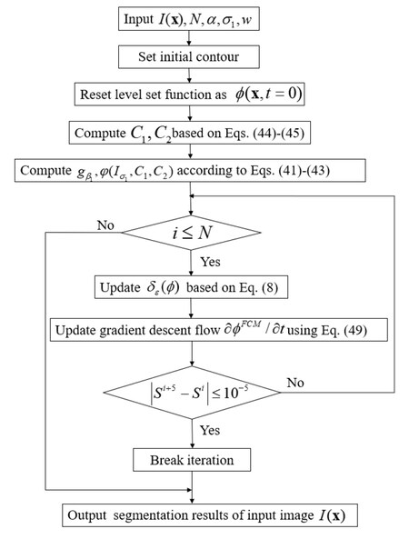
Figure 1. The flow chart of FCM model.
FCM model is characterized by pre-fitting the fuzzy two centroids inside and outside the contour line using the local area-based fuzzy C-mean clustering principle before iteration to construct an adaptive edge indicator function, which solves the one-way motion problem of the edge level set model. However, FCM algorithm applied in this model is unoptimized and complex, which results in relatively long segmentation time. In addition, segmentation may fail in the forms of falling into false boundaryboundaries, if FCM algorithm has poor performance.
3.3. Hybrid ACMs
3.3.1. Optimized local pre-fitting image model
To achieve better segmentation accuracy and reduce computation cost, OLPFI model [70] is proposed to associate region-based attributes and edge-based attributes through mean local pre-fitting functions, which is capable of effectively segments segmenting images with uneven intensity and noise disturbance.
OLPFI energy function is defined as
Note that
where
There are
In Equation (50), the local pre-fitted image (LPFI) function is defined as
with
where
Note that the global minimizer can be computed point by point by simply solving
In order to improve segmentation performance, Equation (54) is rewritten as
where
In order to effectively regularize the level set function and smooth evolution curve, a regularization function
where the regularization function
In Equation (58)
where
3.3.2. re-fitting energy model
To obtain better segmentation precision and decrease CPU elapsed time, PFE model [49] combines median pre-fitting functions with optimized adaptive functions, which solves the issue of unidirectional motion of evolution curve and hugely decreases computation cost.
PFE energy function is constructed as
where
Note that
with
where
In Equation (64),
Note that
The single potential function
The evolution speed function
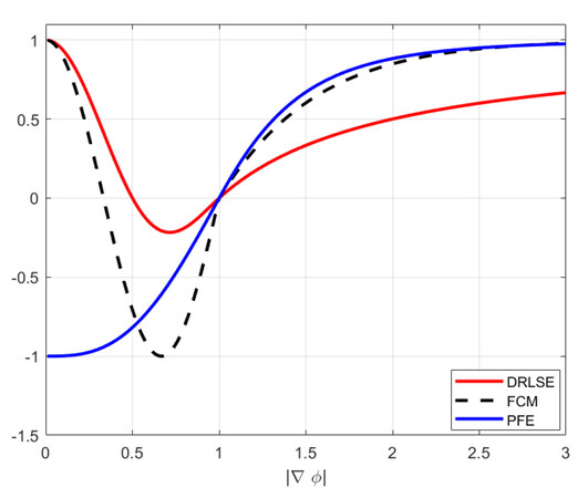
Figure 2. Contrast of DRLSE, FCM, PFE models on evolution speed equations
Applying the steepest descent approach to minimize the energy function in Equation (60), which achieves the following gradient descent flow function as
In Equation (68), the gradient descent flow function consists of three parts. The first part denotes internal energy
PFE model combines energy function based on median pre-fitting functions with adaptive functions, which realizes and accelerates the bidirectional evolution of contour line and reduces the probability of edge leakage. In addition, this model is able to effectively handle images with uneven intensity. However, the issues of falling into false boundary boundaries and insufficient segmentation at the boundary edge may sometimes happen while segmenting images with a large target.
4. EXPERIMENTAL RESULTS
Different kinds of ACMs have been reviewed in Section
Common evaluation criteria for assessing different segmentation approaches are segmentation time and segmentation quality. The authors evaluate segmentation time through the CPU running time
Note that
4.1. Dataset characteristic
All images utilized in this paper are downloaded from a public open source image library called Berkeley segmentation data set and Benchmarks 500 (BSDS500), which can be reached on the website https://www2.eecs.berkeley.edu/Research/Projects/CS/vision/bsds/ for more details. Specifically, for medical images (a-h) in Figure 4, images (a-b) are blood capillaries, image (c) is CT of bone, images (d) is bacteria embryo, image (e) is kidney, image (f) is the internal structure of the brain, and images (g-h) are B-ultrasound of uterus. For natural images (a-h) in Figure 5, image (a) is a piece of maple leaf, image (b) is a shell, image (c) is a starfish, image (d) is a polar bear, image (e) is a bradypod, image (f) is a stone bench, image (g) is plane, and image (h) is an eagle.
4.2. Segmentation experiment of synthetic images
Intensity non-uniformity and noise interference often occur in image segmentation. In Figure 3, the segmentation results of the
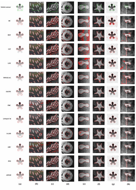
Figure 3. The segmentation results of the first comparative experiment to segment synthetic images. The 1st row represents initial contours, the 2nd to 12th rows denote segmentation results of BC [32], RSF [34], LIF [35], LPF [48], RSF&LoG [39], OLPFI [70], PBC [57], LPF & FCM [41], LGJD [58], ABC [56], PFE [47], and APFJD [49], respectively.
Numerical analysis of segmentation results (The CPU running time
| Image(a)(100 × 100) | Image(b)(132 × 103) | Image(c)(256 × 233) | Image(d)(136 × 132) | Image(e)(103 × 97) | Image(f)(214 × 209) | Image(g)(100 × 100) | Image(h)(127 × 107) | |
| BC | 2.159/20/0.928 | 7.726/180/0.799 | 10.288/200/0.711 | 1.015/30/0.552 | 9.912/200/0.836 | 7.445/180/0.914 | 7.831/180/0.820 | 18.086/300/0.581 |
| RSF | 2.875/300/0.718 | 5.928/300/0.784 | 18.380/300/0.309 | 12.776/220/0.207 | 23.527/500/0.256 | 15.856/300/0.929 | 14.628/300/0.832 | 19.251/300/0.499 |
| LIF | 1.468/200/0.917 | 2.658/150/0.835 | 13.895/200/0.408 | 5.315/180/0.211 | 15.563/200/0.547 | 10.814/200/0.729 | 10.412/200/0.941 | 1.047/120/0.688 |
| LPF | 5.221/300/0.662 | 5.117/300/0.780 | 10.429/500/0.433 | 4.585/220/0.267 | 5.606/300/0.553 | 23.248/500/0.927 | 3.148/150/0.945 | 1.425/120/0.431 |
| RSF&LoG | 5.751/200/0.674 | 6.853/200/0.683 | 10.635/300/0.701 | 4.856/180/0.554 | 7.963/200/0.944 | 20.835/300/0.879 | 4.258/100/0.949 | 1.125/100/0.503 |
| OLPFI | 0.961/60/0.945 | 4.754/200/0.727 | 8.758/200/0.394 | 1.021/60/0.880 | 5.761/200/0.945 | 8.635/200/0.758 | 7.468/180/0.714 | 1.249/65/0.604 |
| PBC | 6.142/300/0.882 | 5.856/300/0.587 | 8.967/300/0.593 | 1.165/90/0.796 | 4.821/200/0.951 | 8.617/300/0.935 | 5.804/200/0.918 | 0.346/65/0.571 |
| LPF & FCM | 3.494/300/0.876 | 5.108/300/0.661 | 7.752/300/0.717 | 0.543/85/0.875 | 3.264/280/0.949 | 9.822/300/0.920/0.958 | 3.365/200/0.913/0.954 | 0.449/60/0.731 |
| LGJD | 3.952/200/0.725 | 4.585/200/0.515 | 5.856/250/0.874 | 3.658/200/0.230 | 8.635/300/0.611 | 7.423/300/0.894 | 10.528/300/0.939 | 1.437/120/0.474 |
| ABC | 0.641/20/0.958 | 6.589/300/0.415 | 15.254/300/0.576 | 0.196/20/0.855 | 8.111/300/0.931 | 3.856/150/0.941 | 5.964/250/0.934 | 7.215/280/0.575 |
| PFE | 2.964/150/0.803 | 3.589/180/0.834 | 5.545/200/0.879 | 0.248/90/0.891 | 3.132/180/0.954 | 12.826/600/0.902 | 3.792/180/0.926 | 0.237/90/0.812 |
| APFJD | 0.855/65/0.917 | 1.856/100/0.795 | 6.982/250/0.820 | 0.285/65/0.838 | 3.915/200/0.936 | 4.570/200/0.878 | 3.253/180/0.924 | 0.958/100/0.610 |
4.3. Segmentation experiment of medical images
ACMs are extensively applied to process medical images to find out the location of the lesion. Consequently, the
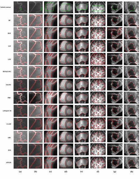
Figure 4. The segmentation results of the second comparative experiment to segment medical images. The 1st row represents initial contours, the 2nd to 12th rows denote segmentation results of BC [32], RSF [34], LIF [35], LPF [48], RSF&LoG [39], OLPFI [70], PBC [57], LPF & FCM [41], LGJD [58], ABC [56], PFE [47], and APFJD [49], respectively.
Numerical analysis of segmentation results (The CPU running time
| Image(a) | Image(b) | Image(c) | Image(d) | Image(e) | Image(f) | Image(g) | Image(h) | |
| BC | ||||||||
| RSF | ||||||||
| LIF | ||||||||
| LPF | ||||||||
| RSF&LoG | ||||||||
| OLPFI | ||||||||
| PBC | ||||||||
| LPF & FCM | ||||||||
| LGJD | ||||||||
| ABC | ||||||||
| PFE | ||||||||
| APFJD |
4.4. Segmentation experiment of natural images
0Bias correction (BC), Region scalable fitting (RSF), Local image fitting (LIF), Local pre-fitting (LPF), Region scalable fitting and optimized Laplacian of Gaussian (RSF&LoG), Optimized local pre-fitting image (OLPFI), Pre-fitting bias field (PBC), Local pre-fitting and fuzzy c-means (LPF & FCM), Local and global Jeffreys divergence (LGJD), Additive bias correction (ABC), Pre-fitting energy (PFE), and Adaptive pre-fitting function and Jeffreys divergence (APFJD).
The
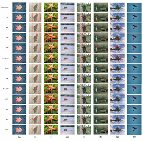
Figure 5. The segmentation results of the third comparative experiment to segment synthetic images. The 1st row represents initial contours, the 2nd to 12th rows denote segmentation results of BC [32], RSF [34], LIF [35], LPF [48], RSF&LoG [39], OLPFI [70], PBC [57], LPF & FCM [41], LGJD [58], ABC [56], PFE [47], and APFJD [49], respectively.
Numerical results of segmentation outcomes (The CPU running time
| Image(a) | Image(b) | Image(c) | Image(d) | Image(e) | Image(f) | Image(g) | Image(h) | |
| BC | ||||||||
| RSF | ||||||||
| LIF | ||||||||
| LPF | ||||||||
| RSF&LoG | ||||||||
| OLPFI | ||||||||
| PBC | ||||||||
| LPF & FCM | ||||||||
| LGJD | ||||||||
| ABC | ||||||||
| PFE | ||||||||
| APFJD |
In Table 3, for image (a), the IOU value of LPF model is the largest while the CPU running time
4.5. Comparison experiments with Deep learning-based algorithms
To compare the segmentation results between ACMs and deep learning-based algorithms, DeepLabv3+ [71] and Mask R-CNN algorithms [72] are selected to segment
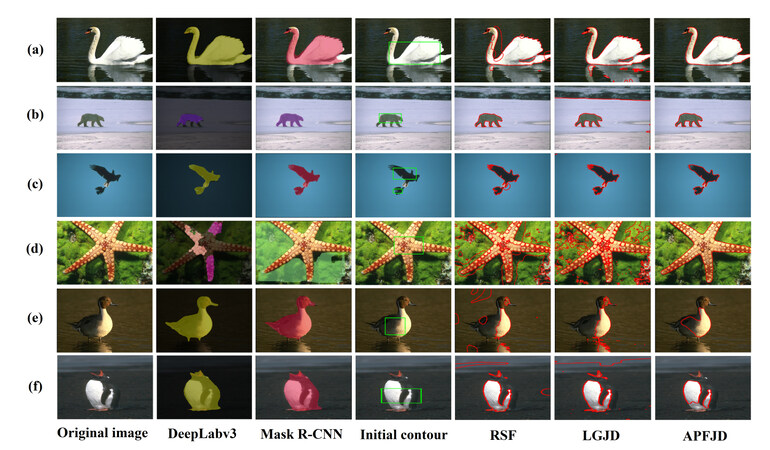
Figure 6. The segmentation results between DeepLabv3+ algorithm [71], Mask R-CNN algorithm [72], RSF [34] model, LGJD [58] model and APFJD [49] model. The 1st column represents original images, the 2nd to 3rd columns signify segmentation results of DeepLabv3+ algorithm and Mask R-CNN algorithm, respectively, the 4th column denotes initial contours of ACMs, and the 5th to 7th columns represent segmentation results of RSF model, LGJD model and APFJD model, respectively.
Numerical analysis of IOUs between DeepLabv3 algorithm, Mask R-CNN algorithm, RSF model, LGJD model, APFJD model in images (a-f) in Figure 6.
| DeepLabv3+ | Mask R-CNN | RSF | LGJD | APFJD | |
| Image a (481 × 321) | |||||
| Image b (481 × 321) | |||||
| Image c (481 × 321) | |||||
| Image d (481 × 321) | |||||
| Image e (481 × 321) | |||||
| Image f (321 × 481) |
In Table 4, for image (a), the DeepLabv3+ algorithm obtains the biggest IOU value due to the most excellent segmentation result. For image (b), the Mask R-CNN algorithm, RSF model and APFJD achieve similar IOU values. For image(c), the RSF model obtains the smallest IOU value due to the issue of edge leakage, and similar results are achieved by the remaining models. For image (d), the DeepLabv3+ and Mask R-CNN algorithms acquire very unsatisfactory IOU values due to failed segmentation. On the contrary, the APFJD model attains the largest IOU value because of clear and clean segmentation. For image (e), the DeepLabv3+ and Mask R-CNN algorithms demonstrate the advantages of segmentation of multi-phase images, which obtains much bigger IOU values than 3 ACMs (RSF, LGJD, APFJD models). The DeepLabv3+ algorithm attains the largest IOU value due to a more fully segmented target. For image (f), the Mask R-CNN algorithm obtains the best segmentation result in terms of the biggest IOU value.
4.6. Summary
Since the images with unevenly distributed intensity, the area inside and outside evolution curves are not intensity uniform. The calculated intensity averages are incapable tocannot represent intensity distribution. Therefore, BC model estimates a bias field to process images with unevenly distributed intensity, which works well with images (a-b) in Figure 3. However, common issues such as falling into false boundary boundaries may occur in images (c-d) in Figure 3. In addition, this model cannot effectively process images with noise interference such as images (e, g, h) in Figure 3. BesidesAdditionally, under- segmentation may take place as image (h) in Figure 3 and images (c, g) in Figure 4 shows. In addition, BC model leaks from target boundary when it segments natural images, as the second row in the Figure 5 indicates.
RSF model is capable of segmenting images with uneven intensity as image (b) in Figure 3. However, the incorporated kernel function only computes the gray values of image local image regions, which makes it easy to fall into a local minimum during the process of energy minimization such as images (a, c) in Figure 3. Nevertheless, falling into a false area still remains unsolved as images (c, d, g) in Figure 3. In addition, the segmentation time is long due to at least four convolution operations to update fitting functions during each iteration. BesidesIn addition, this model has poor anti-noise ability, which is vulnerable to the influence of noise interference, as images (e, g, h) illustrate. Moreover, the issues of under- segmentation and leaking from weak edge still exists, as shown in images (c, e) in Figure 4 and images (g, h) in Figure 4, respectively. Lastly, this model obtains poor segmentation results when segmenting natural images, as shown in the third row in the Figure 5.
Compared with RSF model, LIF model only utilizes two convolution operations to update fitting functions, which greatly reduces the CPU running time T and iteration number N according to Tables
LPF model locally computes average image intensity ahead of iteration process, which reduces the computation cost to some degree. However, the Gaussian kernel function is also used in this model to update the level set function, which results in falling into false boundary boundaries (as described in image (a) in Figure 3) and edge leakage (as illustrated in images (b, c, d) in Figure 3). In addition, this model has further improved in terms of anti-noise ability as shown in images (f, g) in Figure 3. However, the issue of boundary leakage still exists in images (e, h) in Figure 3 and images (g, h) in Figure 4 and images (e, f, g, h) in Figure 5. Besides, the problem of trapping into false boundary boundaries still occurs in images (b, c) in Figure 5.
RSF&LoG model combines RSF model and Laplacian of Gaussian (LoG) energy to smooth the homogeneous areas and enhance boundary characteristics simultaneously to segment images with uneven intensity, which can segment images with uneven intensity to some extent. However, this model may create some common issues such as under- segmentation and falling into false boundary boundaries in images (a, b, c) in Figure 3 and images (d, h) in Figure 3, respectively. In addition, boundary leakage may occur in some cases (as shown in image (h) in Figure 4 and images (c, e) in Figure 5).
OLPFI model calculates the mean intensity of the selected local regions before iteration starts, which dramatically decreases segmentation time. This model puts region-based attributes and edge-based attributes together to handle images with intensity non-uniformity, which obtains excellent results as shown in image (a, d) in Figure 3. However, under- segmentation often occurs in images (b, c, f, g, h) in Figure 3, image (e) in Figure 4, and images (a, g, h) in Figure 5. this This model has relatively poor anti-noise ability in the form of under- segmentation as indicated in images (f, g, h) in Figure 3. Lastly, this model greatly reduces the possibility of boundary leakage and falling into fake false boundaryboundaries.
PBC model utilizes the optimized FCM algorithm to estimate the bias field before iteration process, which gets rid of time-consuming convolution operation during each iteration and greatly reduces segmentation time. In addition, this model can segment images with uneven intensity in images (a, d) in Figure 3. However, boundary leakage may occur in some cases (as indicated in images (b, c) in Figure 3). Moreover, this model is capable of effectively segmenting images with noise interference with high segmentation quality. Nevertheless, under- segmentation may occur in some cases (as indicated in images (h) in Figure 3, image (e) in Figure 4 and images (a, e) in Figure 5). Lastly, falling into fake false boundary boundaries may take place in some cases (as shown in images (b, c) in Figure 5).
LPF & FCM model employs the FCM algorithm and adaptive sign function to solve the issue of boundary leakage, which obtains outstanding performance to segment images with intensity non-uniformity in images (a, d) in Figure 3. However, issues such as under- segmentation and falling into local minima may occur in some cases (as shown in images (b, c) in Figure 3 and images (b, c, g) in Figure 5, respectively). In addition, this model has strong robustness to images with noise (as indicated in images (e-h) in Figure 3). Lastly, this model is capable of effectively segmenting medical images (a-h) in Figure 4 with high accuracy.
LGJD model utilizes the changeable weights to control the local and global data fitting energies based on Jeffreys divergence (JD), which is capable of segmenting images with intensity non-uniformity to some degree. However, this model also has common issues such as over- segmentation or under- segmentation in some cases (as shown in images (a, b, c) in Figure 3 and images (e, f, g) in Figure 5). In addition, boundary leakage may occur during the process of segmenting images with noise interference in some cases (as illustrated in image (e, h) in Figure 3). Besides, the issue of strapping into false boundary boundaries frequently takes place in some cases (as shown in images (d) in Figure 3, images (g, h) in Figure 4, and images (a-d) in Figure 5).
ABC model applies the theory of bias field to segment images with unevenly distributed intensity, which obtains excellent segmentation performance in terms of handling images with intensity non-uniformity in images (a, d) in Figure 3. However, this model has issues of leaking from weak boundary boundaries in some cases (as illustrated in images (b, c) in Figure 3). In addition, this model can effectively handle images with noise interference due to the effect of additive bias correction as shown in images (e, f, g) in Figure 3. Nevertheless, the problem of under- segmentation may happen in image (h) in Figure 4 and images (a, c) in Figure 5. Lastly, this model is also able to effectively segment medical images (a-h) in Figure 4 with high precision.
PFE model computes the median intensity of the chosen local areas ahead of iteration process, which greatly reduces computation cost. According to the twelfth row of Figure 3, this model is able to deal with images with uneven intensity and has excellent noise resistivity. However, common issues such as falling into fake false boundary boundaries and boundary leakage may take place in some cases (as indicated in image (c) in Figure 3 and images (b, c, g) in Figure 5). Lastly, this model is also competent to effectively segment medical images (a-h) in Figure 4 with high efficiency.
APFJD model computes average intensity of selected areas before iteration takes place, which dramatically decreases segmentation time. This model can effectively segment images with uneven intensity and noise interference due to the effect of JD, as shown in images (a-b, d) and images (e-f) in Figure 3. However, the issue of strapping into false boundary boundaries may happen as indicated in image (c) in Figure 3). In addition, under- segmentation may occur in some cases (as indicated in image (e) in Figure 3 and image (c, f) in Figure 4). Lastly, this model segments natural images (a-h) in Figure 5 with excellent accuracy.
To conclude the characteristic of above said ACMs, the calculation processes of BC, RSF, LIF, LPF, RSF&LoG, and LGJD models are too complex to be implemented in practice, which have poor anti-noise capability and spend a huge amount of time for curve evolution. In addition, the computation processes to compute pre-fitting functions in OLPFI, PBC, PFE, and APFJD models are optimized, which enables them to quickly segment different kinds of images within a short amount of time. LPF & FCM takes advantages of FCM clustering to divide the input image region into background region and foreground region before iteration begins, which greatly reduces the computational overhead. ABC model implements K-means
Although ACMs can effectively segment double-phase images with fair segmentation results, the majority of existing ACMs are not able to segment multi-phase images as indicated in images (e, f) in Figure 6. Note that double-phase image means a target in an image either contains black pixels or white pixels, while multi-phase image means a target in an images contains black and white pixels at the same time as shown in images (e, f) in Figure 6. According to Figure 6, the deep learning-based algorithms (DeepLabv3+ and Mask R-CNN algorithms) exhibit an advantage on in segmenting multi-phase images. Specifically, ACMs (RSF, LGJD, APFJD models) can barely segment multi-phase images (e, f) in in Figure 6, while DeepLabv3+ and Mask R-CNN algorithms obtain excellent segmentation results in terms of much bigger IOU value. However, failed segmentation in the form of under- segmentation may take placeoccur while implementing DeepLabv3+ and Mask R-CNN algorithms to segment double-phase images as illustrated in images (b, d) in Figure 6.
5. CHALLENGES AND PROMISING FUTURE DIRECTIONS
Nowadays, there are still various common issues waiting for solutions in the field of image segmentation in practice. The review of the above ACMs points out some common issues and concludes some promising future directions. It is believed that this discussion will be useful for later researchers in this field to design more advanced models.
5.1. The combination of deep learning models
Inspired by the general idea of ACMs, the work [73-75] incorporates region and length constraint terms into the cost or loss function of convolutional neural network (CNN) model based on traditional Dense U-Net for image segmentation, which combines geometric attributes such as edge length with region information to achieves better segmentation accuracy. In addition, compared with traditional ACMs requiring iterations to solve PDEs, the employment of CNN greatly reduces computation cost in image segmentation, although its training process is generally long. In addition, later researchers embed some loss functions in deep learning [76-81] in region-based level set energy functions to improve segmentation efficiency and accuracy. Therefore, one can put the energy function of diverse ACMs mentioned in this paper and other segmentation models in deep learning together to design some new hybrid energy functions to further improve segmentation performance, which is recommended as a promising future research direction in the area of image segmentation.
5.2. The combination of edge-based and region-based ACMs
As discussed in this paper, active contour method can be grouped into two types: the region-based ACM and the edge-based ACM. The region-based ACM utilizes a pre-defined region descriptor or a contour representation to recognize each region on the image, while the edge-based ACM uses the differential property or gradient information of boundary points to construct a contour representation. The region-based ACMs generally utilize regional information (the pixel grayscale information) of the image to construct energy functions, which improves their system robustness and effectiveness. However, the region-based ACMs cannot deal with contours that do not evolve from region boundaries. The edge-based ACMs mainly use the gradient information of the target boundary points as the main driving force to guide the motion of the evolution curve, which is capable of handling topology changes adaptively. Nevertheless, the edge-based ACMs generally need to reinitialize the level set function periodically during the evolution process, which will affect the computational accuracy and slow down segmentation efficiency. In this case, the zero level set may not be able to move towards the target boundary, and how and when to initialize it still remains unsolved.
Therefore, it is necessary to combine the strengths of the region-based and region-based ACMs to obtain better segmentation outcomes. Recently, several hybrid ACMs [41,47,70,82,83] are constructed to take advantage of both metrics of the region-based and edge-based ACMs to achieve higher segmentation efficiency and lower computation cost. It is recommended that future researchers design more hybrid ACMs on the basis of the hybrid ones mentioned above.
5.3. Fast and stable optimization algorithm
The general optimization process of ACMs is to minimize the associated energy function through gradient or steepest descent method. However, it should be aware that it may be hard to figure out the global minima if the energy function is non-convex [33,84-87], which may cause a failed segmentation in the form of falling into a local minima. Specifically, the traditional gradient or steepest descent approach is initialized by the initial level set function and then descends at each iteration, ; the descending direction is controlled by the slope or the derivative of the evolution curve. It is possible to replace the traditional one with other gradient descent methods to design a brand-new series of ACMs, which is capable of optimizing the evolution curve and avoiding falling into local minima.
6. CONCLUSIONS
This paper has presented an overview of different kinds of ACMs in image segmentation in Sections
DECLARATIONS
Authors' contributions
Writing- Original draft preparation: Chen Y, Ge P
Writing-Reviewing and Editing: Wang G, Weng G
Conceptualization: Chen Y, Wang G, Chen H
Methodology: Chen Y, Wang G, Chen H
Project administration: Chen Y, Wang G
Recourses: Chen Y, Chen H
Supervision: Weng G, Chen H
Data curation: Chen Y, Ge P
Software: Ge P, Weng G
Investigation: Ge P
Visualization: Ge P
Availability of data and materials
Not applicable.
Financial support and sponsorship
This research paper was supported in part by National Natural Science Foundation of China under Grant 62103293, in part by Natural Science Foundation of Jiangsu Province under Grant BK20210709, in part by Suzhou Municipal Science and Technology Bureau under Grant SYG202138, and in part by Entrepreneurship and Innovation Plan of Jiangsu Province under Grant JSSCBS20210641.
Conflicts of interest
All authors declared that there are no conflicts of interest.
Ethical approval and consent to participate
Not applicable.
Consent for publication
Not applicable.
Copyright
© The Author(s) 2023.
REFERENCES
1. Son LH, Tuan TM. Dental segmentation from X-ray images using semi-supervised fuzzy clustering with spatial constraints. Eng Appl of Art Int 2017;59:186-95.
2. Civit-Masot J, Luna-Perejón F, Corral JMR, et al. A study on the use of Edge TPUs for eye fundus image segmentation. Eng Appl Art Int 2021;104:104384.
3. Akbari Y, Hassen H, Al-Maadeed S, Zughaier SM. COVID-19 lesion segmentation using lung CT scan images: comparative study based on active contour models. Applied Sciences 2021;11:8039.
4. Guo Q, Wang L, Shen S. Multipleʜchannel local binary fitting model for medical image segmentation. Chin J Electron 2015;24:802-6.
5. Zhang D, Li J, Li X, Du Z, Xiong L, Ye M. Local—global attentive adaptation for object detection. Eng Appl Art Int 2021;100:104208.
6. Yang C, Wu L, Chen Y, Wang G, Weng G. An active contour model based on retinex and pre-Fitting reflectance for fast image segmentation. Symmetry 2022;14:2343.
7. Chen H, Liu Z, Alippi C, Huang B, Liu D. Explainable intelligent fault diagnosis for nonlinear dynamic systems: from unsupervised to supervised learning. IEEE Trans Neur Netw Lear Syst 2022;Early Access.
8. Ge P, Chen Y. An automatic detection approach for wearing safety helmets on construction site based on YOLOv5. In: 2022 IEEE 11th Data Driven Control and Learning Systems Conference (DDCLS). IEEE; 2022. pp. 140-45.
9. Cao Y, Wang G, Yan D, Zhao Z. Two algorithms for the detection and tracking of moving vehicle targets in aerial infrared image sequences. Remote Sensing 2016;8:28.
11. Paragios N, Deriche R. Geodesic active contours and level sets for the detection and tracking of moving objects. IEEE Trans Pattern Anal Machine Intell 2000;22:266-80.
12. Wu Z, Tian E, Chen H. Covert attack detection for LFC systems of electric vehicles: a dual time-varying coding method. IEEE/ASME Trans Mechatron 2022:1-11.
13. Cootes TF, Edwards GJ, Taylor CJ. Active appearance models. IEEE Trans Pattern Anal Machine Intell 2001;23:681-85.
14. Mille J. Narrow band region-based active contours and surfaces for 2D and 3D segmentation. Compu Vis Image Und 2009;113:946-65.
16. Tsai A, Yezzi A, Willsky AS. Curve evolution implementation of the Mumford-Shah functional for image segmentation, denoising, interpolation, and magnification. IEEE Trans Image Process 2001;10:1169-86.
17. Wang G, Zhang F, Chen Y, Weng G, Chen H. An active contour model based on local pre-piecewise fitting bias corrections for fast and accurate segmentation. IEEE Trans Instrum Meas 2023;72:1-13.
18. Xiang Y, Chung ACS, Ye J. An active contour model for image segmentation based on elastic interaction. J Comput Phys 2006;219:455-76.
19. Huang AA, Abugharbieh R, Tam R. A Hybrid Geometric—Statistical Deformable Model for Automated 3-D Segmentation in Brain MRI. IEEE Trans Biomed Eng 2009;56:1838-48.
20. Pluempitiwiriyawej C, Moura JMF, Wu YJL, Ho C. STACS: new active contour scheme for cardiac MR image segmentation. IEEE Trans Med Imaging 2005;24:593-603.
21. Bowden A, Sirakov NM. Active contour directed by the poisson gradient vector field and edge tracking. J Math Imaging Vis 2021;63:665-80.
22. Fahmi R, Jerebko A, Wolf M, Farag AA. Robust segmentation of tubular structures in medical images. In: Reinhardt JM, Pluim JPW, editors. SPIE Proceedings. SPIE; 2008. pp. 691443-1443-7.
23. Zhang H, Morrow P, McClean S, Saetzler K. Coupling edge and region-based information for boundary finding in biomedical imagery. Pattern Recogn 2012;45:672-84.
24. Wen J, Yan Z, Jiang J. Novel lattice Boltzmann method based on integrated edge and region information for medical image segmentation. Biomed Mater Eng 2014;24:1247-52.
25. Lv H, Zhang Y, Wang R. Active contour model based on local absolute difference energy and fractional-order penalty term. Appl Math Model 2022;107:207-32.
26. Mumford D, Shah J. Optimal approximations by piecewise smooth functions and associated variational problems. Comm Pure Appl Math 1989;42:577-685.
27. Caselles V, Catte F, Coll T, Dibos F. A geometric model for active contours in image processing. Numer Math 1993;66:1-31.
29. Bresson X, Esedoglu S, Vandergheynst P, Thiran JP, Osher S. Fast global minimization of the active contour/snake model. Math Imaging Vis 2007;28:151-67.
30. Cohen LD, Kimmel R. Global minimum for active contour models: a minimal path approach. Int J Compu Vis 1997;24:57-78.
31. Li C, Xu C, Gui C, Fox MD. istance regularized level set evolution and its application to image segmentation. IEEE Trans Image Process 2010;19:3243-54.
32. Li C, Huang R, Ding Z, et al. A level set method for image segmentation in the presence of intensity inhomogeneities with application to MRI. IEEE Trans Image Process 2011;20:2007-16.
33. Li C, Kao CY, Gore JC, Ding Z. Implicit active contours driven by local binary fitting energy. In: 2007 IEEE Conference on Computer Vision and Pattern Recognition. IEEE; 2007. pp. 1-7.
34. Li C, Kao CY, Gore JC, Ding Z. Minimization of region-scalable fitting energy for image segmentation. IEEE Trans Image Process 2008;17:1940-9.
35. Zhang K, Song H, Zhang L. Active contours driven by local image fitting energy. Pattern Recogn 2010;43:1199-206.
36. Chan TF, Esedoglu S, Nikolova M. Algorithms for finding global minimizers of image segmentation and denoising models. SIAM J Appl Math 2006;66:1632-48.
37. Chambolle A, Cremers D, Pock T. A convex approach to minimal partitions. SIAM J Imaging Sci 2012;5:1113-58.
38. Wang L, Li C, Sun Q, Xia D, Kao CY. Active contours driven by local and global intensity fitting energy with application to brain MR image segmentation. Comput Med Imaging Graph 2009;33:520-31.
39. Ding K, Xiao L, Weng G. Active contours driven by region-scalable fitting and optimized Laplacian of Gaussian energy for image segmentation. Signal Proce 2017;134:224-33.
40. Wang L, He L, Mishra A, Li C. Active contours driven by local Gaussian distribution fitting energy. Signal Proce 2009;89:2435-47.
41. Jin R, Weng G. Active contours driven by adaptive functions and fuzzy c-means energy for fast image segmentation. Signal Proce 2019;163:1-10.
42. Liu S, Peng Y. A local region-based Chan—Vese model for image segmentation. Pattern Recogn 2012;45:2769-79.
43. Liu W, Shang Y, Yang X. Active contour model driven by local histogram fitting energy. Pattern Recognit Lett 2013;34:655-62.
44. Wang H, Huang TZ, Xu Z, Wang Y. An active contour model and its algorithms with local and global Gaussian distribution fitting energies. Inform Sciences 2014;263:43-59.
45. Ji Z, Xia Y, Sun Q, Cao G, Chen Q. Active contours driven by local likelihood image fitting energy for image segmentation. Inform Sciences 2015;301:285-304.
46. Yang Y, Ren H, Hou X. Level set framework based on local scalable Gaussian distribution and adaptive-scale operator for accurate image segmentation and correction. Signal Processing: Image Communication 2022;104:116653.
47. Ge P, Chen Y, Wang G, Weng G. A hybrid active contour model based on pre-fitting energy and adaptive functions for fast image segmentation. Pattern Recogn Lett 2022;158:71-79.
48. Ding K, Xiao L, Weng G. Active contours driven by local pre-fitting energy for fast image segmentation. Pattern Recogn Lett 2018;104:29-36.
49. Ge P, Chen Y, Wang G, Weng G. An active contour model driven by adaptive local pre-fitting energy function based on Jeffreys divergence for image segmentation. Expert Syst Appl 2022;210:118493.
50. Liu G, Jiang Y, Chang B, Liu D. Superpixel-based active contour model via a local similarity factor and saliency. Measurement 2022;188:110442.
51. Chen H, Zhang H, Zhen X. A hybrid active contour image segmentation model with robust to initial contour position. Multimed Tools Appl 2022 sep.
52. Yang Y, Hou X, Ren H. Efficient active contour model for medical image segmentation and correction based on edge and region information. Expert Syst Appl 2022;194:116436.
53. Zhang W, Wang X, You W, et al. RESLS: Region and edge synergetic level set framework for image segmentation. IEEE Trans Image Process 2020;29:57-71.
54. Dong B, Weng G, Jin R. Active contour model driven by Self Organizing Maps for image segmentation. Expert Syst Appl 2021;177:114948.
55. Fang J, Liu H, Liu J, et al. Fuzzy region-based active contour driven by global and local fitting energy for image segmentation. Applied Soft Comput 2021;100:106982.
56. Weng G, Dong B, Lei Y. A level set method based on additive bias correction for image segmentation. Expert Syst Appl 2021;185:115633.
57. Jin R, Weng G. A robust active contour model driven by pre-fitting bias correction and optimized fuzzy c-means algorithm for fast image segmentation. Neurocomputing 2019;359:408-19.
58. Han B, Wu Y. Active contour model for inhomogenous image segmentation based on Jeffreys divergence. Pattern Recogn 2020;107:107520.
59. Asim U, Iqbal E, Joshi A, Akram F, Choi KN. Active contour model for image segmentation with dilated convolution filter. IEEE Access 2021;9:168703-14.
60. Costea C, Gavrea B, Streza M, Belean B. Edge-based active contours for microarray spot segmentation. Proce Compu Sci 2021;192:369-75.
61. Fang J, Liu H, Zhang L, Liu J, Liu H. Region-edge-based active contours driven by hybrid and local fuzzy region-based energy for image segmentation. Inform Sciences 2021;546:397-419.
62. Yu H, He F, Pan Y. A novel segmentation model for medical images with intensity inhomogeneity based on adaptive perturbation. Multimed Tools Appl 2019;78:11779-98.
63. Sirakov NM. A new active convex hull model for image regions. J Math Imaging Vis 2006;26:309-25.
64. Osher S, Sethian JA. Fronts propagating with curvature-dependent speed: Algorithms based on Hamilton-Jacobi formulations. J Compu Phys 1988;79:12-49.
65. Kass M, Witkin A, Terzopoulos D. Snakes: active contour models. Int J Comput Vision 1988;1:321-31.
66. Bresson X, Vandergheynst P, Thiran JP. A variational model for object segmentation using boundary information and shape prior driven by the mumford-shah functional. Int J Comput Vision 2006;68:145-62.
67. Deriche M, Amin A, Qureshi M. Color image segmentation by combining the convex active contour and the Chan Vese model. Pattern Anal Applic 2019;22:343-57.
68. Aubert G, Kornprobst P. Mathematical problems in Image Processing. New York: Springer; 2006.
69. Wang Y, He C. An adaptive level set evolution equation for contour extraction. Appl Math Comput 2013;219:11420-29.
70. Yan X, Weng G. Hybrid active contour model driven by optimized local pre-fitting image energy for fast image segmentation. Appl Math Model 2022;101:586-99.
71. Chen LC, Zhu Y, Papandreou G, Schroff F, Adam H. Encoder-Decoder with Atrous Separable Convolution for Semantic Image Segmentation. European Conference on Computer Vision 2018 Feb.
72. He K, Gkioxari G, Dollar P, Girshick R. Mask R-CNN. arXiv 2017 Mar.
73. Chen X, Williams BM, Vallabhaneni SR, et al. Learning active contour models for medical image segmentation. In: 2019 IEEE/CVF Conference on Computer Vision and Pattern Recognition (CVPR). IEEE; 2019. pp. 11624-32.
74. Ma J, He J, Yang X. Learning geodesic active contours for embedding object global information in segmentation CNNs. IEEE Trans Med Imaging 2021;40:93-104.
75. Gu J, Fang Z, Gao Y, Tian F. Segmentation of coronary arteries images using global feature embedded network with active contour loss. Comput Med Imaging Graph 2020;86:101799.
76. Gur S, Wolf L, Golgher L, Blinder P. Unsupervised microvascular image segmentation using an active contours mimicking neural network. In: 2019 IEEE/CVF International Conference on Computer Vision (ICCV). IEEE; 2019. pp. 10721-30.
77. Kim B, Ye JC. Mumford—Shah Loss Functional for Image Segmentation With Deep Learning. IEEE Trans Image Process 2020;29:1856-66.
78. Tao H, Qiu J, Chen Y, Stojanovic V, Cheng L. Unsupervised cross-domain rolling bearing fault diagnosis based on time-frequency information fusion. J Franklin Ins 2023;360:1454-77.
79. Chen H, Li L, Shang C, Huang B. Fault detection for nonlinear dynamic systems With consideration of modeling errors: a data-Driven approach. IEEE Trans Cybern 2022:1-11.
80. Qu F, Tian E, Zhao X. Chance-Constrained
81. Chen Y, Jiang W, Charalambous T. Machine learning based iterative learning control for non-repetitive time-varying systems. Int J Robust Nonlinear 2022;Early Veiw.
82. Han B, Wu Y. A hybrid active contour model driven by novel global and local fitting energies for image segmentation. Multimed Tools Appl 2018;77:29193-208.
83. Yang X, Jiang X, Zhou L, Wang Y, Zhang Y. Active contours driven by Local and Global Region-Based Information for Image Segmentation. IEEE Access 2020;8:6460-70.
84. Chen Y, Zhou Y. Machine learning based decision making for time varying systems: Parameter estimation and performance optimization. Knowledge-Based Systems 2020;190:105479.
85. Chen Y, Zhou Y, Zhang Y. Machine Learning-Based Model Predictive Control for Collaborative Production Planning Problem with Unknown Information. Electronics 2021;10:1818.
86. Chen H, Chai Z, Dogru O, Jiang B, Huang B. Data-Driven Designs of Fault Detection Systems via Neural Network-Aided Learning. IEEE Trans Neur Net Lear Syst 2021:1-12.
87. Jiang W, Chen Y, Chen H, Schutter BD. A Unified Framework for Multi-Agent Formation with a Non-repetitive Leader Trajectory: Adaptive Control and Iterative Learning Control. TechRxiv 2023 jan.
Cite This Article
Export citation file: BibTeX | RIS
OAE Style
Chen Y, Ge P, Wang G, Weng G, Chen H. An overview of intelligent image segmentation using active contour models. Intell Robot 2023;3(1):23-55. http://dx.doi.org/10.20517/ir.2023.02
AMA Style
Chen Y, Ge P, Wang G, Weng G, Chen H. An overview of intelligent image segmentation using active contour models. Intelligence & Robotics. 2023; 3(1): 23-55. http://dx.doi.org/10.20517/ir.2023.02
Chicago/Turabian Style
Chen, Yiyang, Pengqiang Ge, Guina Wang, Guirong Weng, Hongtian Chen. 2023. "An overview of intelligent image segmentation using active contour models" Intelligence & Robotics. 3, no.1: 23-55. http://dx.doi.org/10.20517/ir.2023.02
ACS Style
Chen, Y.; Ge P.; Wang G.; Weng G.; Chen H. An overview of intelligent image segmentation using active contour models. Intell. Robot. 2023, 3, 23-55. http://dx.doi.org/10.20517/ir.2023.02
About This Article
Copyright

Data & Comments
Data


 Cite This Article 64 clicks

 Like This Article 56
likes
Like This Article 56
likes


Comments
Comments must be written in English. Spam, offensive content, impersonation, and private information will not be permitted. If any comment is reported and identified as inappropriate content by OAE staff, the comment will be removed without notice. If you have any queries or need any help, please contact us at support@oaepublish.com.