
UAV maneuver decision-making via deep reinforcement learning for short-range air combat


Abstract
The unmanned aerial vehicle (UAV) has been applied in unmanned air combat because of its flexibility and practicality. The short-range air combat situation is rapidly changing, and the UAV has to make the autonomous maneuver decision as quickly as possible. In this paper, a type of short-range air combat maneuver decision method based on deep reinforcement learning is proposed. Firstly, the combat environment, including UAV motion model and the position and velocity relationships, is described. On this basic, the combat process is established. Secondly, some improved points based on proximal policy optimization (PPO) are proposed to enhance the maneuver decision-making ability. The gate recurrent unit (GRU) can help PPO make decisions with continuous timestep data. The actor network's input is the observation of UAV, however, the input of the critic network, named state, includes the blood values which cannot be observed directly. In addition, the action space with 15 basic actions and well-designed reward function are proposed to combine the air combat environment and PPO. In particular, the reward function is divided into dense reward, event reward and end-game reward to ensure the training feasibility. The training process is composed of three phases to shorten the training time. Finally, the designed maneuver decision method is verified through the ablation study and confrontment tests. The results show that the UAV with the proposed maneuver decision method can obtain an effective action policy to make a more flexible decision in air combat.
Keywords
1. INTRODUCTION
The unmanned aerial vehicle (UAV) has been applied in many fields for its low cost and high efficiency, including the military domain[1, 2]. As sensors, artificial intelligence (AI) and other related technologies are developed and applied to UAV, the serviceable range of UAV in the military has been significantly expanded[3]. Air combat is one of the fields where the UAV is utilized.
The air combat is incredibly complex due to the difficulty of predicting the various scenarios that may arise unpredictably. During the combat, especially in short-range air combat, the UAV performs violent maneuvers which make the combat scenarios change instantly. There are roughly three categories of methods, optimization methods, game theory methods and AI methods, to solve the short-range air combat maneuver decision-making problem[3, 4]. For the optimization methods, the maneuver decision problem is turned into an optimization problem, and solved by the optimization theories, like optimization algorithms[4, 5]. However, the optimization problem for air combat is a high-dimensional and large-scale problem that is usually so difficult and complex that most optimization-based decision-making algorithms cannot be executed in real-time and adapt to practical constraints. Game theory methods, especially differential games[6, 7], are another popular method to solve air combat maneuver decision problems. Whereas, the mathematical models of game theory methods are difficult to establish and their solutions are always hard to prove the adequacy and necessity[4]. For the complex air combat problem, AI methods catch the scholars for their flexibility and operability. The expert system method[8] is one of the AI methods, which tries to map the human knowledge and experience into the flight rule library to complete the maneuver decision. However, the mapping process is complex because human knowledge and experience are always hard to generalize into rules and describe mathematically. On the other hand, once the rule library has been built, the maneuver policy is fixed and inflexible[3]. The methods based on reinforcement learning (RL) are popular for air combat problems recently.
RL is a type of machine learning method that improves its action policy with respect to the reward obtained by repeated trial and error in an interactive environment[9]. In recent years, the neural network has been combined with RL, which is called deep reinforcement learning (DRL). Many types of DRL algorithms have been proposed, like deep Q network (DQN), deep deterministic policy gradient (DDPG), proximal policy optimization (PPO), etc. DRL has been applied in UAV path control[10], quadrupedal locomotion control[11], autonomous platoon control[12], etc. At the same time, DRL has been used to improve the operational efficiency of air combat[9, 13, 14]. In ref.[3], the DQN is used to solve one-to-one short-range air combat with an evaluation model and maneuver decision model, and basic-confrontation training is presented because of the huge computation load. The PPO is used to learn the continuous 3-DoF short-range air combat strategy in ref.[15], and it can adapt to the combat environment to beat the enemy who uses the minmax strategy. With the DRL method, the UAV can adapt to the changing combat situation and make a reasonable maneuver decision. However, the huge computation load and slow training speed are still the main issues that needs to be addressed when combining DRL with air combat problems.
In this paper, the problem of one-to-one UAV short-range air combat maneuver decision-making is studied. The main contributions are summarized as follows.
(1) The air combat environment with the attacking and advantage areas is designed to describe the relationship between the UAVs. And to increase the confrontment difficulty, the attacking conditions, blood values and the enemy action policy consisting of prediction and decision are introduced.
(2) The GRU layer is applied to design the neural networks which are used as the PPO's actor and critic networks. On the other hand, the observation of the UAV for actor network and combat state information for critic network are designed to separate their roles.
(3) To improve flexibility and intelligence during the confrontment, the reward function is divided into three parts: dense reward, event reward and end-game reward. Then, the phased training process is designed from easy to difficult to ensure the feasibility of training.
The remainder of this paper is organized as follows. In section II, the UAV motion model, air combat environment and its process are introduced. Then the method designed is explained in section III, which includes the PPO algorithm, some improved points and the design for state, action and reward function to combine the PPO algorithm with the air combat problem. The action policy for the enemy and training process is also introduced. Next, the training results and simulation analysis are presented in section IV. Finally, the conclusion is presented in section V.
2. PROBLEM FORMULATION
2.1. UAV motion model
The three-degree-of-freedom UAV model is considered because the main consideration in short-range air combat problem is the position and velocity relationship between the two sides[3]. The motion model is established in the ground coordinate system as East-North-Up (ENU) coordinate system, which is shown in Figure 1.
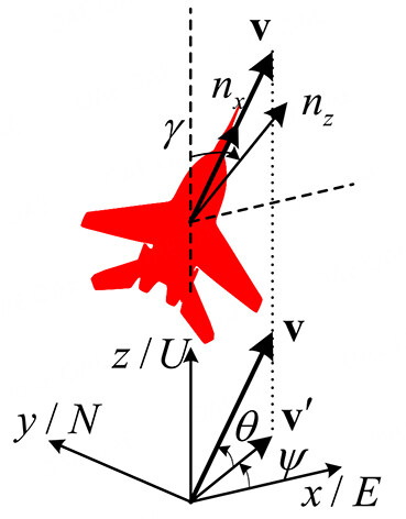
Figure 1. The UAV's motion model in the ground coordinate system. UAV: unmanned aerial vehicle
To simplify the problem, assume that the velocity direction is fixed with the -axis of the body coordinate system, and the UAV's motion model is shown as[14, 16]
where
where subscript
By giving the control parameters' values and UAV's state at the time step
2.2. Air combat environment
In the one-to-one short-range air combat environment, there are two UAVs, divided into red and blue. The red aims to gain the advantage situation over the blue until the blue side is destroyed by its weapon, and the blue aims to do the opposite[4]. In this paper, the red UAV is controlled by the proposed decision method based on DRL algorithm. The relationship between the red and blue sides during the battle, which is shown in Figure 2, is mainly described by both sides' velocity vectors, the red's velocity
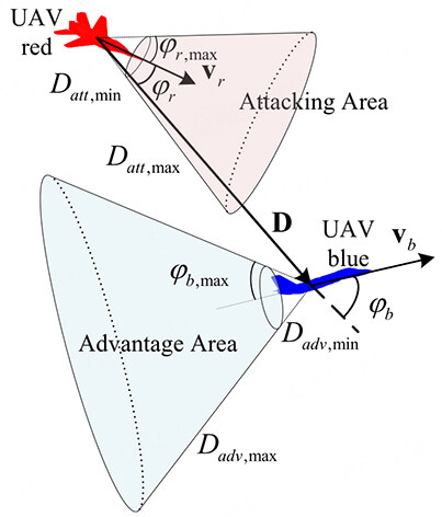
Figure 2. The relationship between the red and blue sides during the battle.
where
The angle
During the confrontation, the red has a chance to attack and deal damage to the blue only if the blue is in its attacking area.
where
The angle
During the confrontation, the red not only needs to keep the blue in its attacking area but also tries to avoid being attacked by the blue. Thus, the advantage area for the red is defined behind the blue and can be described as
where
During air combat, the UAV has limited attacking resource and needs attack only under certain conditions. The enemy should be both within the red's attacking area and hard to escape. These conditions can be described as[15]
where
where
Note that Figure 1 is shown from the red perspective, and the relative relationship between the two sides can also be defined from the blue perspective in the same way. In the view of the blue, distance vector
2.3. Air combat process
For an episode of one-to-one short-range air combat, the red and the blue are initiated, then confront in the combat environment until the conditions for the end of the episode are satisfied[17]. An episode ends when the red or the blue is damaged or the maximum decision step
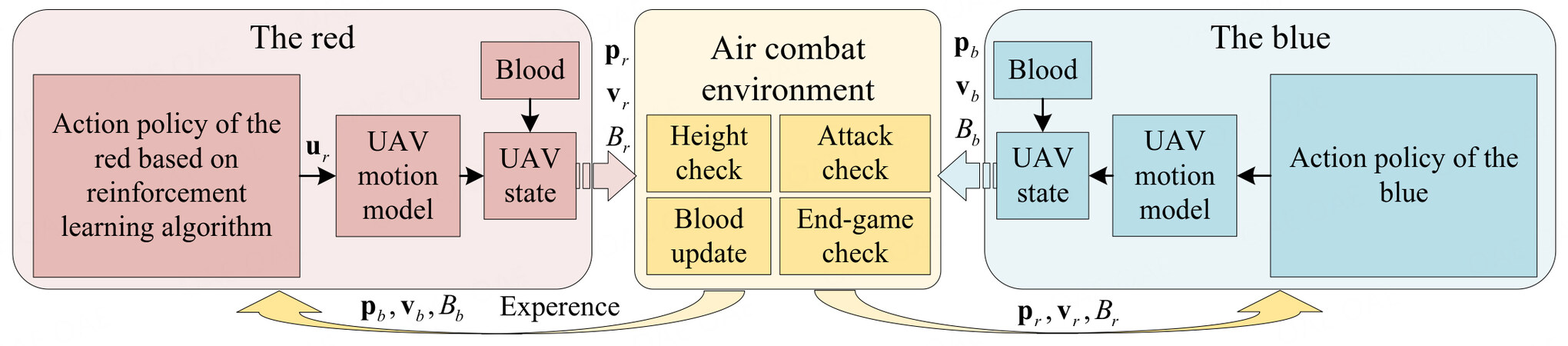
Figure 3. Short-range air combat framework.
Algorithm 1 Air combat process in an episode Input: position:
Output: confrontation result in the view of the red
1. for all
2: set
3: use the red's action policy to get
4: use the blue's action policy to get
5: update the red's and the blue's positions and velocities by Equation (1)
6: if
7: set
8: end if
9: if
10: set
11: end if
12: if
13: calculate
14: if satisfy Equation (8) then
15: get a random number
16: calculate
17: set
18: end if
19: end if
20: if
21: calculate
22: if satisfy Equation (10) then
23: get a random number
24: calculate
25: set
26: end if
27: end if
28: if
29: set
30: return red win
31: else if
32: set
33: return red loss
34: else if
35: set
36: return tie
37: else if
38: set
39: return tie
40: else
41: set
42: end if
43: end for
3. AIR COMBAT DECISION METHOD DESIGN
3.1. PPO algorithm and improvement
The PPO algorithm is a type of DRL algorithm that has been used in many types of problems. In this part, the basic PPO algorithm and its usage in short-range air combat are introduced.
3.1.1. The PPO algorithm
The PPO algorithm is based on the actor-critic framework and the policy gradient method (PG), which can be applied to continuous or discrete motion space problems.[18] PG-based algorithms maximize the action policy's expected return by updating the action policy directl[19]. The PPO algorithm's main objective is[18]
where
where
where
In this paper, the red's action policy is based on the PPO algorithm. Thus,
Algorithm 2 The usage of the PPO algorithm in short-range air combat
1: initialize the PPO's hyperparameters, including epoch
2: initialize the air combat environment including the UAVs' positions, velocities, blood values, etc.
3: initialize the number of experiences in experience buffer
4: for all
5: execute the process shown in Algorithm 1, including updating the UAVs' positions, velocities, blood values and damage flags. For each time step,
6: if
7: calculate the return for every step and normalize the advantage
8: set
9: for all
10: sample from the experience buffer based on the batch size
11: calculate the loss of each batch by Equation (11)
12: update the networks' parameters by Adam optimizer
13: set
14: end for
15: set
16: end if
17: end for
3.1.2. Improved points
To improve the training effect, some improvement points are adopted in this paper, and the framework of PPO algorithm for short-range air combat is shown in Figure 4.
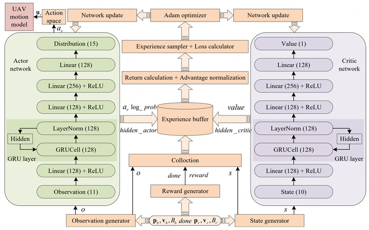
Figure 4. The PPO algorithm framework for short-range air combat.
The first improvement point is considering the historical combat data when making decision. During the confrontation, the red must gradually accumulate the situational advantages over the blue and finally beat it. Therefore, decision on current action should take into account the previous air combat situations. The link between the action decision and historical air combat experience is established by adding the gate recurrent unit (GRU)[22] to the neural network. The GRU is a type of recurrent neural network (RNN), which can adaptively capture the time's dependencies in different scales[22], similar to long short-term memory (LSTM). However, the GRU is easier to train and more efficient than LSTM. The GRU layer, the hidden layer using GRU, is used in both actor network and critic network. The networks' inputs, observation and state, are firstly processed by the fully connected network to extract the inputs' features. Then the features are fused with historical features by the GRU layer to obtain the integrated features considering the historical situational features. The specific process is shown in Figure 4.
The second improvement point is to differentiate the neural network inputs. For the basic PPO algorithm, the critic network uses the same input as the actor network, which is named state space[20]. However, the actor and critic networks play different roles in the algorithm. The actor network's state space is in the view of the red because the actor network's input is the red's observation of the air combat environment. On the other hand, the critic network is used to evaluate the output of the actor network by its output, the critic value, based on the current air combat situation[23]. Thus, the input of critic network can be more objective and include some information that cannot be observed by the red. In this vein, the observation
The third improvement point is a variable-sized experience buffer. For each time step, the experiences are stored in the experience buffer in order. During the training, it is divided into thousands of episodes, and each episode is over if it satisfies the ending condition. Thus, the length of each episode may be different. To make the training more general, the network parameters are updated until enough experiences are stored. However, the return calculation should be calculated on the basis of the complete experiences. Therefore, when the networks are updated, the numbers of experiences, which are larger than the number of the minimum experience for training
The fourth improvement point is the phased training process, which is discussed in section 3.6.
3.2. State space design
The state space of air combat should contain the information of the red and the blue UAVs, and a suitable designed state space can speed up the convergence of training. In this part, two state spaces designed for actor network and critic network are introduced.
3.2.1. The actor network's state space
The designed state space consists of two parts, position information
The
where the subscript
where
At the same time, to avoid the difference between the values of each state variable from being too large to affect the learning efficiency of the network, the normalization for every state variable is adopted. The threshold vector
where
where
3.2.2. The critic network's state space
The actor network gets action according to the relationship in the view of the red, but the critic network gets the evaluation value based on the state of the air combat environment, which can include the information that cannot be observed. Thus, the input for the critic network
where subscript
Then, the
3.3. Action space design
In the air combat problem, the UAV's actions are always summed up as a maneuver library, which consists of a series of tactical actions, such as high yo-yo, cobra maneuvering and so on[3]. Pilots can choose from the library according to the combat situation. However, the establishment of the library is difficult and complex, and these tactical actions can be disassembled into basic actions. Thus, fifteen basic actions
The basic action's values in the designed action space
| No. | Action | Values for | No. | Action | Values for |
| 1 | Forward, maintain | 0; 1; 0 | 2 | Forward, accelerate | 2; 1; 0 |
| 3 | Forward, decelerate | -1; 1; 0 | 4 | Upward, maintain | 0; 3.5; 0 |
| 5 | Upward, accelerate | 2; 3.5; 0 | 6 | Upward, decelerate | -1; 3.5; 0 |
| 7 | Downward, maintain | 0; -3.5; 0 | 8 | Downward, accelerate | 2; -3.5; 0 |
| 9 | Downward, decelerate | -1; -3.5; 0 | 10 | Left turn, maintain | 0; 3.5; arccos (2/7) |
| 11 | Left turn, accelerate | 2; 3.5; arccos (2/7) | 12 | Left turn, decelerate | -1; 3.5; arccos (2/7) |
| 13 | Right turn, maintain | 0; 3.5; - arccos (2/7) | 14 | Right turn, accelerate | 2; 3.5; - arccos (2/7) |
| 15 | Right turn, decelerate | -1; 3.5; - arccos (2/7) |
3.4. Reward function design
The aim of RL is to maximize the cumulative reward obtained from the environment. Therefore, the reward function is the bridge to communicate the training result requirements to the DRL algorithm and its design is extremely important[25]. In this paper, the reward function is well-designed and divided into three parts: dense reward, event reward and end-game reward. Different types of rewards are triggered under different conditions to transmit different expectations. In this part, the reward function designed for short-range air combat is introduced.
3.4.1. Dense reward
The red receives a dense reward from the air combat environment after completing the action for every step. Thus, a properly designed dense reward can improve the red's exploration efficiency and speed up the training process. The dense reward is based on the air combat situatio[16] after the execution of the red's and blue's actions and can be considered as the immediate situation value for the maneuvering decision-making. The dense reward
where
where
where
where
As for
3.4.2. Event reward
During air combat, there are many types of events[24, 26], such as attacking successfully, reaching the advantage area, making the enemy in the attacking area and so on. By continuously triggering these events, the red will beat the blue finally. Thus, the event reward is necessary to make the red consciously trigger these events to maintain the advantage. This paper designs two types of event rewards: advantage area reward
where
3.4.3. End-game reward
During the training, the draw result is regarded as a case in which the red loses and is used to motivate the red to beat the blue. When the flag
where
3.5. Action policy for the Blue
During the training, a policy is adopted as the blue's action policy, which consists of prediction and decision. In the prediction step, the blue will predict which action the red will do at the next time step and then estimate the red's position and velocity at the next time step based on the predicted action. At the decision step, the blue will find which action it should take to confront the red. To find which action is better, the thread function
Noting that the definitions of
Algorithm 3 Action policy of the blue Input: position:
Output: the blue's action
1: initialize the thread set
2: for all action
3: calculate the red's
4: calculate thread value by Equation (32) in the view of the red with
5: append the thread value to
6: end for
7: set
8: set
9: calculate the red's
10: initialize the thread set
11: for all action
12: calculate the blue's
13: calculate thread value by Equation (32) in the view of the blue with
14: append the thread value to
15: end for
16: set
17: set
18: return
3.6. Training process
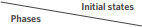
In the confrontation training, the red and the blue confront each other for thousands of episodes in the air combat environment. Every episode works as Algorithm 1 and for every step the blue makes the maneuver decision as Algorithm 3. To train the red's action policy with the DRL algorithm, the experience for every step is stored. When satisfying the training conditions, the experiences will be used to update the red's action policy. To make sure the training is successful and to obtain satisfactory results, the training is divided into three phases, basic, dominant and balanced[3]. The initial states for these phases are shown in Table 2.
The initial states of the UAVs in three training phases
 | Camp | ||||||
| Basic | Red | 60 | 0 | ||||
| Blue | 60 | 0 | |||||
| Dominant | Red | 60 | 0 | ||||
| Blue | 60 | 0 | |||||
| Balanced | Red | 60 | 0 | ||||
| Blue | 60 | 0 |
The three phases constitute a progressive relationship, which means the later training is based on the training results of the former training. The red's actor network and critic network are loaded with the former trained networks' parameters before starting the training.
4. RESULTS
4.1. Parameters setting
The hyperparameters setting for the DRL algorithm is shown in Table 3[18].
The hyperparameters setting for the DRL algorithm
| Hyperparameter | Value | Hyperparameter | Value |
| Learning rate | 0.00025 | GAE paramerter | 0.95 |
| Discount | 0.99 | Minimum buffer size | |
| Number of batches | 4 | Epoch | |
| Clip parameter | 0.1 | Main objective's coefficients |
The parameters of the designed air combat environment are set as follows[15]. For the attacking distance, it is set as
4.2. Training results in the phases
The four cases are trained with the hyperparameters in Table 3 and initial states in Table 2. Four cases are compared in this paper, which are case I PPO, case II PPO with GRU, case III PPO with GRU and state input and case IV PPO with state input. The state input means the inputs of actor and critic networks are different, and if there is no GRU, the GRU layer in Figure 4 is replaced with linear layer with 128 units and ReLU.
In the basic phase, the UAVs' states are shown in the first line of Table 2. The blue always performs the forward and maintain action
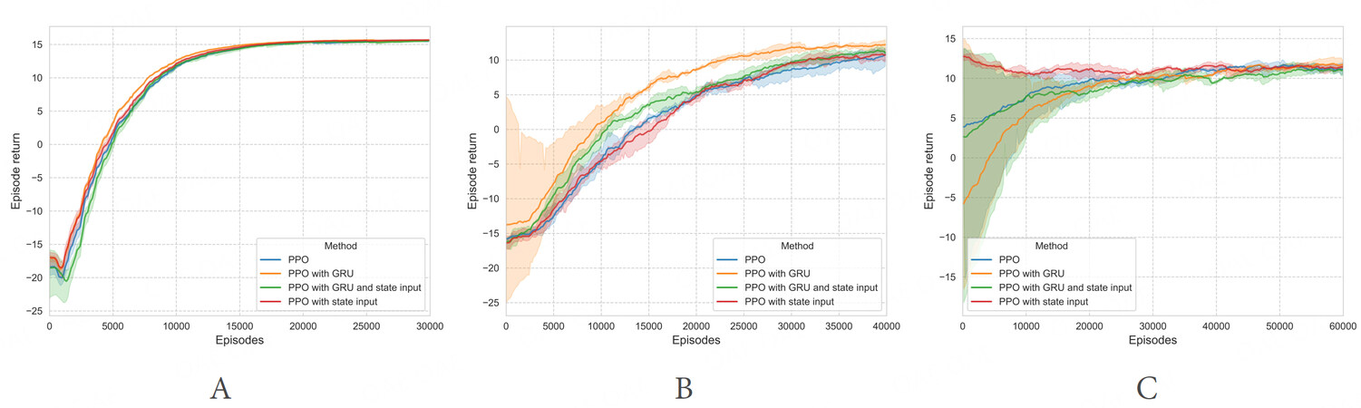
Figure 5. The episode returns of every episode in the three phases while training. A: the episode returns in the basic phase; B: the episode returns in the dominant phase; C: the episode returns in the balanced phase.
It can be seen that the PPO algorithm can go to converge faster when it is combined with GRU. In the basic phase, a relatively simple scenario, all four cases can easily find a better action policy to enclose the blue and beat it. And in the more complex scenario, it can find a better policy faster with GRU. But there are also larger episode reward variations in its infancy. Therefore, the state input is introduced to reduce the episode reward variations, which will synchronize to slightly reduce the final episode reward.
In addition, to test the final training result for the four cases, the training results in the balanced phase are reloaded and the initial states of the UAVs are set as
And the maneuvering trajectories are shown in Figure 6. The steps for the four cases are 146, 90, 123 and 193. For Figure 6B, it is shown that the blue and the red collide. It is obvious that the red can beat the blue in a smaller space range when trained with PPO with GRU, and by adding state input, the red can be more flexible to avoid collision. But the cost is the increase in time steps, which explains the decrease of final episode reward. In case III, the red uses hover and altitude variations to lure the blue closer and gain an advantage situation, instead of pursuing the blue.
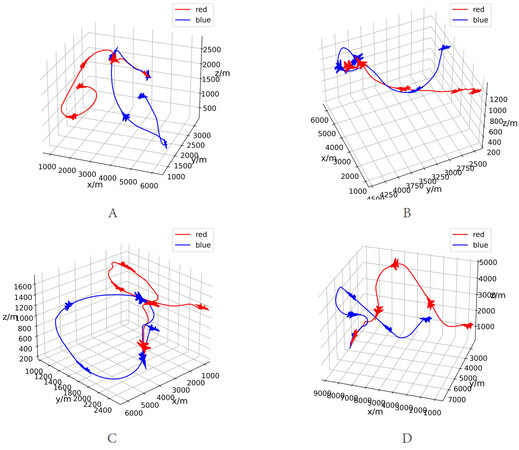
Figure 6. The maneuvering trajectories in the training test for four cases. A: the maneuvering trajectories for the case I PPO; B: maneuvering trajectories for case II PPO with GRU; C: maneuvering trajectories for case III PPO with GRU and state input; D: maneuvering trajectories for case IV PPO with state input.
4.3. Confrontation tests
To compare the final training result of four cases, the confrontation tests for the four cases are conducted in this part when all of the training is finish. To accelerate the confrontation tests, the
The confrontment test results between four cases
| Algorithm case | Results (100 episodes) | |||
| Win rate | Loss rate | Tie rate | ||
| Tie win rate | Tie loss rate | |||
| PPO with GRU and state input vs. PPO | 74% | 12% | 9% | 5% |
| PPO with GRU and state input vs. PPO with GRU | 57% | 1% | 17% | 25% |
| PPO with GRU and state input vs. PPO with state input | 52% | 14% | 14% | 20% |
It can be seen that by combining PPO with GRU and state input, the UAV can get a more flexible and intelligent action policy even though the training process is the same. It is proved that training the action policy by the PPO with proposed improve points can help the UAV gain an advantage situation more quickly and greater operational capability in short-range air combat confrontation, and the action policy can be more intelligent to adapt to the blue's uncertain policy.
5. CONCLUSIONS
In this article, a maneuver decision method for UAV air combat is proposed based on the PPO algorithm. To enhance the PPO's performance, the GRU layer and different compositions of networks' inputs are adopted. At the same time, to accelerate training, some designs are applied. The action space is discretized into 15 basic actions, and the reward function is well-designed with three parts. Further, the training process is divided into several progressively more complex phases. To illustrate the advantages of the designed method, ablation experiments and UAV air combat tests are conducted in this paper. The episode rewards and confrontment test results show that the designed maneuver decision method can generate a more intelligent action policy for the UAV to win short-range air combat. By combining the PPO with the improved points, the training feasibility is improved and convergence is more efficient. The proposed maneuver decision-making method is always is able to achieve a win rate of more than 50% and a loss rate of less than 15%.
In future, the more complex six-degree-of-freedom UAV motion model and tighter UAV performance constraints could be introduced to improve accuracy. On the other hand, the multiple-to-multiple air combat problem, including multi-UAV coordinated attacking and tactical decisions, is the focus of future research.
DECLARATION
Authors' contributions
Made substantial contributions to the research, idea generation, software development, and conduct the DRL experiments. Wrote and edited the original draft: Zheng Z
Performed process guidance responsibility for the planning and execution of the study, as well as the evolution of overarching research aims, critical review, and material support. Review and revise the original draft: Duan H
Availability of data and materials
Not applicable.
Financial support and sponsorship
This work was partially supported by National Natural Science Foundation of China under grant #U20B2071, #91948204, #T2121003 and #U1913602.
Conflicts of interest
All authors declared that there are no conflicts of interest.
Ethical approval and consent to participate
Not applicable.
Consent for publication
Not applicable.
Copyright
© The Author(s) 2023.
REFERENCES
1. Ayass T, Coqueiro T, Carvalho T, Jailton J, Araújo J, Francês R. Unmanned aerial vehicle with handover management fuzzy system for 5G networks: challenges and perspectives. Intell Robot 2022;2:20-6.
2. Zhang JD, Yang QM, Shi GQ, Lu Y, Wu Y. UAV cooperative air combat maneuver decision based on multi-agent reinforcement learning. J Syst Eng Electron 2021;6:1421-88.
3. Yang QM, Zhang JD, Shi GQ, Hu JW, Wu Y. Maneuver decision of UAV in short-range air combat based on deep reinforcement learning. IEEE Access 2020;8:363-78.
4. Ruan WY, Duan HB, Deng YM. Autonomous maneuver decisions via transfer learning pigeon-inspired optimization for UCAVs in dogfight engagements. IEEE/CAA J Autom Sinica 2022;9:1639-57.
5. Yang Z, Zhou DY, Piao HY, Zhang K, Kong WR, Pan Q. Evasive maneuver strategy for UCAV in beyond-visual-range air combat based on hierarchical multi-objective evolutionary algorithm. IEEE Access 2020;8:46605-23.
6. Xu GY, Liu Q, Zhang HM. The application of situation function in differential game problem of the air combat. 2018 Chinese Automation Congress (CAC); 2018 Nov 30-Dec 2; Xi'an, China. IEEE; 2019. pp. 1190–5.
7. Başpınar B, Koyuncu E. Differential flatness-based optimal air combat maneuver strategy generation. AIAA Scitech 2019 Forum; 2019 Jan 7-11; San Diego, CA, USA. AIAA; 2019. pp. 1–10.
8. Wang D, Zu W, Chang HX, Zhang J. Research on automatic decision making of UAV based on Plan Goal Graph. 2016 IEEE International Conference on Robotics and Biomimetics (ROBIO); 2016 Dec 3-7; Qingdao, China. IEEE; 2016. pp. 1245–9.
10. Zhang YT, Zhang YM, Yu ZQ. Path following control for UAV using deep reinforcement learning approach. Guid Navigat Control 2021;1:2150005.
11. Zhang H, He L, Wang D. Deep reinforcement learning for real-world quadrupedal locomotion: a comprehensive review. Intell Robot 2022;2:275-97.
12. Boin C, Lei L, Yang SX. AVDDPG - Federated reinforcement learning applied to autonomous platoon control. Intell Robot 2022;2:145-67.
13. Li YF, Shi JP, Jiang W, Zhang WG, Lyu YX. Autonomous maneuver decision-making for a UCAV in short-range aerial combat based on an MS-DDQN algorithm. Def Technol 2022;9:1697-714.
14. Li Y, Han W, Wang YG. Deep reinforcement learning with application to air confrontation intelligent decision-making of manned/unmanned aerial vehicle cooperative system. IEEE Access 2020;8:67887-98.
15. Li LT, Zhou ZM, Chai JJ, Liu Z, Zhu YH, Yi JQ. Learning continuous 3-DoF air-to-air close-in combat strategy using proximal policy optimization. 2022 IEEE Conference on Games (CoG); 2022 Aug 21-24; Beijing, China. IEEE; 2022. pp. 616–9.
16. Kang YM, Liu Z, Pu ZQ, Yi JQ, Zu W. Beyond-visual-range tactical game strategy for multiple UAVs. 2019 Chinese Automation Congress (CAC); 2019 Nov 22-24; Hangzhou, China. IEEE; 2019. pp. 5231–6.
17. Ma XT, Xia L, Zhao QC. Air-combat strategy using deep Q-learning. 2018 Chinese Automation Congress (CAC); 2018 Nov 30-Dec 2; Xi'an, China. IEEE; 2019. pp. 3952–7.
18. Schulman J, Wolski F, Dhariwal P, Radford A, Klimov O. Proximal policy optimization algorithms; 2017.
19. Wu JT, Li HY. Deep ensemble reinforcement learning with multiple deep deterministic policy gradient algorithm. Math Probl Eng 2020;2020:1-12.
20. Yuksek B, Demirezen MU, Inalhan G, Tsourdos A. Cooperative planning for an unmanned combat aerial vehicle fleet using reinforcement learning. J Aerosp Inform Syst 2021;18:739-50.
21. Xing JW. RLCodebase: PyTorch codebase for deep reinforcement learning algorithms; 2020. Available from: https://github.com/KarlXing/RLCodebase. [Last accessed on 15 Mar 2023].
22. Chung JY, Gulcehre C, Cho K, Bengio Y. Empirical evaluation of gated recurrent neural networks on sequence modeling; 2014.
23. Pope AP, Ide JS, Micovic D, et al. Hierarchical reinforcement learning for air-to-air combat; 2021.
24. Sun ZX, Piao HY, Yang Z, et al. Multi-agent hierarchical policy gradient for air combat tactics emergence via self-play. Eng Appl Artif Intel 2021;98:104112.
25. Hu JW, Wang LH, Hu TM, Guo CB, Wang YX. Autonomous maneuver decision making of dual-UAV cooperative air combat based on deep reinforcement learning. Electronics 2022;11:467.
26. Jing XY, Hou MY, Wu GL, Ma ZC, Tao ZX. Research on maneuvering decision algorithm based on improved deep deterministic policy gradient. IEEE Access 2022;10:92426-45.
Cite This Article
Export citation file: BibTeX | RIS
OAE Style
Zheng Z, Duan H. UAV maneuver decision-making via deep reinforcement learning for short-range air combat. Intell Robot 2023;3(1):76-94. http://dx.doi.org/10.20517/ir.2023.04
AMA Style
Zheng Z, Duan H. UAV maneuver decision-making via deep reinforcement learning for short-range air combat. Intelligence & Robotics. 2023; 3(1): 76-94. http://dx.doi.org/10.20517/ir.2023.04
Chicago/Turabian Style
Zheng, Zhiqiang, Haibin Duan. 2023. "UAV maneuver decision-making via deep reinforcement learning for short-range air combat" Intelligence & Robotics. 3, no.1: 76-94. http://dx.doi.org/10.20517/ir.2023.04
ACS Style
Zheng, Z.; Duan H. UAV maneuver decision-making via deep reinforcement learning for short-range air combat. Intell. Robot. 2023, 3, 76-94. http://dx.doi.org/10.20517/ir.2023.04
About This Article
Special Issue
Copyright

Data & Comments
Data


 Cite This Article 30 clicks

 Like This Article 9
likes
Like This Article 9
likes


Comments
Comments must be written in English. Spam, offensive content, impersonation, and private information will not be permitted. If any comment is reported and identified as inappropriate content by OAE staff, the comment will be removed without notice. If you have any queries or need any help, please contact us at support@oaepublish.com.