Research Article | Open Access | 30 Mar 2023

Human gait tracking for rehabilitation exoskeleton: adaptive fractional order sliding mode control approach

Views: 599 | Downloads: 500 | Cited:

Yuan Zhou^1,2

, ...

Tian Wang³

Intell Robot 2023;3(1):95-112.

10.20517/ir.2023.05 | © The Author(s) 2023.

Author Information

Article Notes

Cite This Article

Abstract

To improve the rehabilitation training effect of hemiplegic patients, in this paper, a discrete adaptive fractional order fast terminal sliding mode control approach is proposed for the lower limb exoskeleton system to implement high-precision human gait tracking tasks. Firstly, a discrete dynamic model is established based on the Lagrange system discretization criterion for the lower limb exoskeleton robot. Then, in order to design a discrete adaptive fractional order fast terminal sliding mode controller, the Grünwald–Letnikov fractional order operator is introduced to combine with fast terminal attractor to construct a fractional order fast terminal sliding surface. An adaptive parameter adjustment strategy is proposed for the reaching law of sliding mode control, which drives the sliding mode to the stable region dynamically. Moreover, the stability of the control system is proved in the sense of Lyapunov, and the guidelines for selecting the control parameters are given. Finally, the simulations are tested on the MATLAB-Opensim co-simulation platform. Compared with the conventional discrete sliding mode control and discrete fast terminal sliding mode control, the results verify the superiority of the proposed method in improving lower limb rehabilitation training.

Keywords

Lower-limb exoskeleton, adaptive discrete-time sliding mode, fractional order control, finite-time convergence

Download PDF 0 2

1. INTRODUCTION

In recent years, the aging population of many countries in the world has increased sharply, and the health problems of the elderly have been widely concerned by the public ^[1]. Stroke is a common disease in the elderly population, which will lead to the paralysis of the lower limbs of patients. If the patient can get timely and effective exercise rehabilitation treatment, the patient's motor function can be restored ^{[1, 2]}. Traditional rehabilitation training mainly relies on physical therapists to provide patients with highly repetitive training. However, the number of therapists is seriously insufficient to meet the social requirements. Furthermore, the traditional method is a mostly subjective evaluation, which is inefficient and cannot guarantee effectiveness. In this situation, a lower limb exoskeleton robot is useful for the patient to conduct repetitive rehabilitation training, greatly reduce the burden of therapists, and assist doctors in accurately observing patients' rehabilitation status. Generally, rehabilitation can be divided into three stages based on the degree of spinal cord injury: initial, intermediate, and terminal. In the initial stage, due to the weak mobility of the patient, the patient needs to wear the lower limb exoskeleton robot to accurately follow the predetermined gait trajectory for rehabilitation training. With the gradual recovery of mobility, the patient can enter the middle and final stages of active rehabilitation training ^[2]. Therefore, the initial stage is crucial for the entire rehabilitation training. However, the uncertainty and disturbance caused by the unexpected behavior of stroke patients will seriously impact the initial rehabilitation training.

To improve rehabilitation efficiency at the initial stage and eliminate the influence of external disturbance, many control algorithms can be applied to exoskeleton robots. For instance, the PID control, adaptive control, robust control ^[3], fuzzy control ^[4], active disturbance rejection control ^[5], neural network control ^[6], Master-Slave Synchronization ^[7], and sliding mode control methods ^[8]. Among the methods, sliding mode control has the characteristics of fast response, insensitivity to uncertainties, and easy implementation in motion control applications. In particular, the sliding mode control can overcome the problems of external disturbances and uncertainties by constructing the reaching law and sliding mode surface in theory, so that the controlled system can achieve higher tracking accuracy. Non-singular terminal sliding mode control ^[9] and fast terminal sliding mode control ^[10] were applied to overcome parameter uncertainty and external disturbances to realize gait tracking control of lower limb exoskeleton rehabilitation robot, and theoretically analyzed the stability of controller design and tracking accuracy of trajectory. Sliding mode control technology can also be combined with the neural network, a recurrent neural network-based robust nonsingular sliding mode control is proposed for the non-holonomic spherical robot, it can enhance the robustness to control the system ^[11]. To obtain higher accuracy, fractional order sliding mode control is introduced to deal with uncertainties and external disturbances. Fractional order sliding mode control has the characteristics of global memory and elimination of jitter, so it is widely used in industry, such as micro gyroscope ^[12], manipulator control ^[13], and permanent magnet synchronous motor control ^[14]. In addition, the fractional order control algorithm can be applied in the field of robot control in combination with other technical methods. For example, a fractional neural integral sliding-mode controller based on the Caputo-Fabrizio derivative and Riemann–Liouville integral for a robot manipulator mounted on a free-floating satellite ^[15] and a method based on the nested saturations technique and the Caputo-Fabrizio derivative for a quadrotor aircraft ^[16]. In chaotic systems, the application of fractional order can endow the system with more degrees of freedom ^[17], help to study the dynamic behavior of the system, combined with robust control methods ^[18], eliminate external interference, and effectively solve the synchronization problem of the system ^[19]. However, the general fractional order sliding mode control strategy is designed based on the continuous time state of the controlled object and is directly been tested on the digital computer system, so the design of the controller ignoring the sampling interval will lead to the loss of the control system precision ^{[20, 21]}. Moreover, the use of fractional operators to construct sliding mode functions also introduces the influence of uncertainty. If the fractional operators are defined by Gr$$ \ddot{\rm u} $$nwald–Letnikov (GL), there are non-physical initial conditions in the experiment. The fractional definition of Caputo is feasible in engineering applications, but the definition of Caputo can only be implemented in the approximation method based on the Laplace transform, which will introduce additional approximation errors to the control system ^[22].

In this paper, a novel discrete adaptive fractional order fast terminal sliding mode controller (AFOFTSMC) is designed for high-precision gait trajectory tracking tasks. To reduce the difference between theoretical design and practical application of digital computer systems, the controller designed in this paper derived the discrete-time object model based on the Lagrange discretization criterion. In addition, to preserve the global memorability of fractional operators, Gr$$ \ddot{\rm u} $$nwald–Letnikov fractional difference operators are used to construct discrete sliding mode surfaces. Considering the uncertainty of parameters and the boundedness of disturbances, a new adaptive terminal sliding mode approach law is proposed to drive the sliding mode dynamics to the region of finite step size. In this paper, the theoretical analysis of the system entering the stable state in finite time is given, and the validity of the algorithm is tested on the co-simulation platform of MATLAB and Opensim software.

The rest of this article is structured as follows. The second part describes the lower extremity exoskeleton discrete model based on the Lagrange system discrete criterion. The design and stability analysis of the discrete adaptive fractional order fast terminal sliding mode controller is presented in Section III. In Section IV, the simulation results are analyzed to prove the effectiveness of the controller. Section V summarizes the thesis.

2. DYNAMICS MODEL OF LOWER LIMB EXOSKELETON

The swing leg dynamic model is considered according to a two-degree-of-freedom (2-DOF) lower limb exoskeleton diagram shown in Figure 1. Based on the motion mechanism of human lower limbs, the hip and knee joints are designed as active joints, and the ankle joint is designed as a passive joint. The physical parameters of the 2-DOF lower limb exoskeleton in Figure 1 are explained as follows. $$ O(0,0) $$ represents the coordinate origin, $$ q_i $$$$ (i = 1,2) $$ denotes the angle of the hip or knee joint, $$ l_{ci} $$$$ (i = 1,2) $$ represents the distance between the centroid of thigh or shank segment and the hip joint or knee joint, $$ l_i $$$$ (i = 1,2) $$ corresponds to the length of the thigh or shank segment, $$ m_i $$$$ (i = 1,2) $$ denotes the mass of thigh or shank segment.

$Human gait tracking for rehabilitation exoskeleton: adaptive fractional order sliding mode control approach$

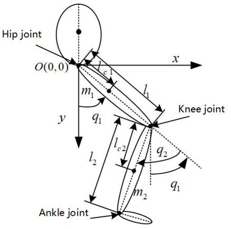
Figure 1. Simplified diagram of 2-DOF lower limb exoskeleton. 2-DOF: two-degree-of-freedom.

To achieve high-precision motion control of the lower limb exoskeleton rehabilitation robot. We established a dynamic model of the lower limb exoskeleton using the Lagrange equation of motion. The equation of general forms is expressed as follows ^[23]:

(1)

$$ \begin{eqnarray} L=T-V \end{eqnarray} $$

(2)

$$ \begin{equation} \tau=\frac{d}{dt}(\frac{\partial{L}}{\partial\dot{q}})-\frac{\partial{L}}{\partial{q}} \end{equation} $$

where $$ L $$ denotes the Lagrangian, $$ T $$ and $$ V $$ represent kinetic energy and potential energy respectively. $$ \tau $$ represents the torque of the system.

The equations of motion of a lower limb exoskeleton robot are described according to the Lagrange equation (2):

(3)

$$ \begin{equation} M(q)\ddot{q}+C(q,\dot{q})\dot{q}+G(q)+N(q,\dot{q},\ddot{q})=\tau \end{equation} $$

where $$ q $$, $$ \dot{q} $$ and $$ \ddot{q} $$ denote the joint angle, angular velocity, and angular acceleration vectors respectively, $$ M(q) \in R^{2\times{2}} $$ is the positive definite inertia matrix, $$ C(q,\dot{q}) \in R^{2\times{2}} $$ is the Coriolis and centrifugal force matrix, $$ G(q) \in R^{2\times{1}} $$ is the gravity matrix ^[3], $$ \tau \in R^{2} $$ is the torque vector, $$ N(q,\dot{q},\ddot{q}) \in R^{2\times{1}} $$ denotes the uncertainty of model parameters and external disturbances. $$ N(q,\dot{q},\ddot{q}) $$ can be expressed as:

(4)

$$ \begin{equation} N(q,\dot{q},\ddot{q})={\Delta}M(q)\ddot{q}+{\Delta}C(q,\dot{q})\dot{q}+{\Delta}G(q)-\tau_{d}. \end{equation} $$

The uncertainty of model parameters and external disturbances should be considered in the actual lower limb exoskeleton dynamics model. $$ {\Delta}M(q) \in R^{2\times{2}} $$, $$ {\Delta}C(q,\dot{q}) \in R^{2\times{2}} $$, $$ {\Delta}G(q) \in R^{2\times{1}} $$ denotes the uncertain inertia part, uncertain Coriolis and centrifugal force part, uncertain gravitational part respectively, and the external disturbances as $$ \tau_d \in R^{2\times{1}} $$.

To design digital motion control systems, it is crucial to obtain nominal discretization dynamics. In this paper, the discretization substitution criterion of the Lagrangian system is used to discretize the dynamics model. The discretization criterion is as follows ^[24]:

(5)

$$ \begin{equation} \frac{d}{dt}(\frac{\partial{L}}{\partial\dot{q}_i})\rightarrow \frac{1}{T}[(\frac{\partial{L}}{\partial\dot{q}_i})_{k+1}-(\frac{\partial{L}}{\partial\dot{q}_i})_{k}] \end{equation} $$

(6)

$$ \begin{equation} \frac{\partial{L}}{\partial{q}_i}\rightarrow \frac{1}{2}[\frac{M(q_{k+1})-M(q_{k})}{q_{i,k+1}-q_{i,k}}]\dot{q}_{i,k+1}\dot{q}_{i,k} \end{equation} $$

where $$ T $$ denotes the sampling period, $$ k $$ denotes time step. Then, the explicit form of the discrete dynamics model is derived as follows ^[25]:

(7)

$$ \begin{equation} \begin{aligned} \begin{cases} q_{k+1}=q_k+T\dot{q}_k \\ \dot{q}_{k+1}=M^{-1}(q_k+T\dot{q}_k)M({q}_{k})\dot{q}_{k}+TM^{-1}(q_k+T\dot{q}_k)C(q_k\\ \quad\qquad+T\dot{q}_k,{q}_{k},\dot{q}_{k})\dot{q}_{k}+TM^{-1}(q_k+T\dot{q}_k)\tau_k-\\ \quad\qquad{TM^{-1}}(q_k+T\dot{q}_k)G(q_k+T\dot{q}_k,{q}_{k}) \end{cases} \end{aligned} \end{equation} $$

the description of the system given in (7) can be expressed in state representation form as:

(8)

$$ \begin{equation} x(k+1)=f(k)+b(k){u(k)}+d(k) \end{equation} $$

(9)

$$ \begin{equation} f(k)=\left[ \begin{matrix} I_{2\times{2}} & I_{2\times{2}}T \\ 0_{2\times{2}} & M^{-1}(q_k+T\dot{q}_k)M({q}_{k})+TM^{-1}(q_k+T\dot{q}_k)C-{TM^{-1}}(q_k+T\dot{q}_k)G \\ \end{matrix} \right]x(k) \end{equation} $$

(10)

$$ \begin{equation} b(k)=\left[ \begin{matrix} 0_{2\times{2}} \\ M^{-1}(q_k+T\dot{q}_k) \\ \end{matrix} \right] \end{equation} $$

where, $$ x(k)=[q_{1,k}, q_{2,k}, \dot{q}_{1,k}, \dot{q}_{2,k}]^T $$ is the system state vector, $$ u(k)=[\tau_{1,k}, \tau_{2,k}]^T $$ is the system control input vector, $$ f(k) \in R^{4\times{1}} $$ is the nonlinear state transition matrix, and $$ b(k) \in R^{4\times{2}} $$ is the control matrix, $$ I_{2\times{2}} $$ is represented as the second-order identity matrix, and $$ 0_{2\times{2}} $$ is a second-order zero matrix, $$ d(k) \in R^{4\times{1}} $$ is the set of parameter uncertainties and external disturbances of the system. Assuming that $$ d(k) $$ is bounded, then $$ ||d(k)||\leq{d}_{\rho} $$.

3. CONTROLLER DESIGN AND STABILITY ANALYSIS

In the previous section, we modeled and analyzed the dynamics model of the lower limb exoskeleton robot. In this section, we will design an appropriate controller for the lower limb exoskeleton robot. The design of the controller is divided into five parts, and the process of controller construction, stability proof, and parameter selection are explained completely. Firstly, before introducing the fractional order sliding mode surface, the definition of fractional order needs to be introduced. Fractional order has the advantage of global memorability and plays an important role in the construction of AFOFTSMC. In the second part, the fractional order fast terminal sliding mode surface and adaptive terminal control law is proposed to construct an AFOFTSMC controller for the lower limb exoskeleton robot. In the third part, the stability of the controller is proved in detail, and it is proved that both the sliding mode variables and the system errors can converge in the bounded region. The fourth part gives some guiding opinions on the parameter selection of the controller. Finally, conventional sliding mode control (CSMC) and fast terminal sliding mode control (FTSMC) controllers are designed to compare with AFOFTSMC.

3.1. Preliminaries

In order to design a discrete adaptive fractional order fast terminal sliding mode controller for the lower limb exoskeleton system, the sliding mode surface function should be designed according to the properties of the fractional order operator, and the adaptive sliding mode control law should be designed to form the controller. Therefore, we will elaborate on the basic definition and related nomenclatures of the fractional operator in detail.

$$ \textbf{Definition 1:} $$ The Gr$$ \ddot{\rm u} $$nwald–Letnikov fractional order operator is defined as follows ^[22]:

(11)

$$ \begin{equation} {_a^{GL}D_t^{\lambda}}f(t)=\frac{1}{h^{\lambda}}\sum\limits_{j=0}^{[(t-a)/h]}{(-1)^j}\binom{\lambda }{j}f(t-jh) \end{equation} $$

where $$ \lambda $$ is the arbitrary order of function $$ f(t) $$, the value of $$ \lambda $$ will affect the calculus properties of fractional order operators. When $$ \lambda>0 $$, the fractional order operator is a differentiator, while $$ \lambda<0 $$, the fractional order operator is an integrator ^[19]. $$ a $$ is the initial value of the integral, and generally, zero initial condition can be assumed, that is, $$ a =0 $$. $$ h $$ is the sampling time interval, and $$ \binom{\lambda }{j} $$ is the binomial coefficient. The specific calculation method is as follows:

(12)

$$ \begin{equation} \binom{\lambda }{j}= \begin{cases} 1 & j=0 \\ \frac{\lambda(\lambda-1){\cdots}(\lambda-j+1)}{j!} & j=1,2,3,\ldots \\ \end{cases}. \end{equation} $$

However, storing all motion data to calculate fractional integrals in practical engineering applications consumes hardware resources and makes the calculation inefficient. Therefore, to improve the operation efficiency and ensure the global memory of the fractional operator, the fractional integral can be calculated by storing part of the motion data, as shown below:

(13)

$$ \begin{equation} {_a^{GL}D_t^{\lambda}}f(t)=\frac{1}{h^{\lambda}}\sum\limits_{j=0}^{L}{(-1)^j}\binom{\lambda }{j}f(t-jh) \end{equation} $$

where $$ L $$ represents the limited amount of data stored.

$$ \textbf{Lemma 1} $$^[22]: The sum of binomial coefficients in equation (13) can be expressed by gamma function $$ \Gamma(z)=\int_{0}^{\infty}e^{-t}t^{z-1}dt $$ as:

(14)

$$ \begin{equation} \sum\limits_{j=0}^{L}{(-1)^j}\binom{\lambda }{j}=\frac{\Gamma(L+1-\lambda)}{\Gamma(1-\lambda)\Gamma(L+1)}. \end{equation} $$

3.2. Controller design

To synthesize the advantages of the fractional order sliding mode surface and the fast terminal sliding mode control law to construct the controller, the appropriate fractional order sliding mode surface should be selected. Several fractional order sliding mode surfaces have been described in the literature ^{[8, 12-14, 22]}. Inspired by the above strategies, the discrete fractional order sliding mode surface selected are as follows:

(15)

$$ \begin{equation} s(k)=c_1{e_1(k)}+{e_2(k)}+c_2{D^\lambda}[|e_1(k)|^{\beta}sgn(e_1(k))] \end{equation} $$

where $$ e_1(k)=[x_{d1}(k)-x_1(k),x_{d2}(k)-x_2(k)]^T $$ is the tracking error between the desired position and real position, $$ e_2(k)=[x_{d3}(k)-x_3(k),x_{d4}(k)-x_4(k)]^T $$ is the tracking error between desired velocity and real velocity, $$ x_d(k) \in R^{4\times{1}} $$ is the reference signal vector, $$ c_1=diag(c_{1i}) $$$$ (i = 1,2) $$, $$ c_2=diag(c_{2i}) $$$$ (i = 1,2) $$ are selected constant matrices, $$ 0<\beta=\frac{q_\beta}{p_\beta}<1 $$ with $$ p_\beta $$, $$ q_\beta $$ being both odd positive integers.

Remark 1: For a nonlinear system, when the system state is far from the equilibrium point, the fractional order terminal sliding mode surface proposed by Sun et al.^[22] can ensure that the system converges in a finite time. However, considering that the system state is close to the equilibrium point, the terminal attractor cannot guarantee the fast convergence of the system. In this paper, a linear term $$ c_1{e_1(k)} $$ is introduced into the sliding mode surface, when the system state is close to the equilibrium point, the convergence time is mainly determined by the linear term $$ c_1{e_1(k)} $$, which can accelerate the convergence of the system. Therefore, the sliding mode surface designed in this paper not only makes the system state converge in a finite time but also preserves the rapidity of the linear sliding mode when it is close to the equilibrium point.

To make the system stable, for the system model (8), the ideal quasi-sliding mode band should meet the following requirements: $$ s(k+1)=0 $$, then the controller can be obtained as follows:

(16)

$$ \begin{equation} C_1=\left[ \begin{matrix} c_{11} & 0 & 1 & 0 \\ 0 & c_{12} & 0 & 1 \\ \end{matrix} \right] \end{equation} $$

(17)

$$ \begin{equation} C_1[x_d(k+1)-f(k)-b(k)u(k)-d(k)]+c_2{D^\lambda}[|e_1(k)|^{\beta}sgn(e_1(k))]=0. \end{equation} $$

The equivalent control law is:

(18)

$$ \begin{equation} u_{eq}(k)=[C_1b(k)]^{-1}[C_1(x_d(k+1)-f(k))+c_2{D^\lambda}[|e_1(k)|^{\beta}sgn(e_1(k))]]. \end{equation} $$

To eliminate the influence brought by system parameter uncertainty and external disturbance, the new adaptive terminal sliding mode reaching law used for system model (8) is:

(19)

$$ \begin{equation} s(k+1)=PQs(k)-TP\Phi|s(k)|^{\alpha}sgn[s(k)] \end{equation} $$

where, $$ P=diag(P_i) $$ with $$ P_i=1-exp\left(-[\frac{s_i(k)}{\epsilon}]^{2m}\right) $$, $$ Q=diag(Q_i) $$ with $$ Q_i=1-\sigma_{i}T $$, $$ \Phi=diag(\Phi_i) $$ with $$ \Phi_i=\delta|s_i(k)| $$, $$ \delta>0 $$, $$ 0<1-\sigma_iT<1 $$, $$ 0<\alpha<1 $$, $$ \epsilon $$ and $$ m $$ are positive real numbers, $$ i=1,2 $$.

Then the switching control law $$ u_{sw} $$ is as follows:

(20)

$$ \begin{equation} \begin{aligned} u_{sw}(k) =-[C_1b(k)]^{-1}[PQs(k)-TP\Phi|s(k)|^{\alpha}sgn[s(k)]]. \end{aligned} \end{equation} $$

Combining (8), (15) and the reaching law (19), an AFOFTSMC law is obtained, and the corresponding control input can be expressed as

(21)

$$ \begin{equation} u(k)=u_{eq}(k)+u_{sw}(k). \end{equation} $$

Substituting equation (21) into the sliding mode function $$ s(k+1) $$, which can be written as:

(22)

$$ \begin{equation} \begin{aligned} s(k+1) =PQs(k)-TP\Phi|s(k)|^{\alpha}sgn[s(k)]-{\xi}(k) \end{aligned} \end{equation} $$

where $$ {\xi}(k)=C_1{d(k)} $$, $$ |{\xi}(k)|\leq \rho_{f} $$, $$ |{\xi}_i(k)|\leq \rho_{i} $$.

3.3. Stability analysis

$$ \textbf{Lemma 2} $$^[20]: If $$ 0<\alpha<1 $$, $$ \psi(\alpha) $$ is a function in equation (23), then $$ \psi(\alpha)-x\psi(\alpha)-1+x^{\alpha}\psi(\alpha)^{\alpha}\geq0 $$ holds for any $$ x\in[0,1] $$.

(23)

$$ \large \begin{equation} \psi(\alpha)=1+\alpha^{\frac{\alpha}{1-\alpha}}-\alpha^{\frac{1}{1-\alpha}} \end{equation} $$

with $$ 0\leq\alpha\leq1 $$, $$ 1<\psi(\alpha)<2 $$.

Proof: Let $$ f(x)=\psi(\alpha)-x\psi(\alpha)-1+x^{\alpha}\psi(\alpha)^{\alpha} $$, then to prove whether the minimum value of $$ f(x) $$ is greater than zero. From the properties of $$ \psi(\alpha) $$, we know that $$ \psi(\alpha)>1 $$, then $$ F(1)=-1+\psi(\alpha)^{\alpha}>0 $$, and $$ f(0)=\psi(\alpha) $$. Then, the extreme value of $$ f(x) $$ can be obtained from $$ \dot{f}(x)=0 $$. When $$ \dot{f}(x)=0 $$, $$ x={\alpha}^{\frac{1}{1-\alpha}}(\psi(\alpha))^{-1} $$ can be obtained, and then the minimum value

$$ f(x)=\psi(\alpha)-{\alpha}^{\frac{1}{1-\alpha}}-1+{\alpha}^{\frac{\alpha}{1-\alpha}}=\psi(\alpha)-1+(\frac{1}{\alpha}-an){\alpha}^{\frac{1}{1-\alpha}}>0 $$

, then the prove is completed.

$$ \textbf{Lemma 3} $$^[20]: If $$ 0<\alpha<1 $$, $$ \psi(\alpha) $$ is a function in equation (23), then $$ \psi(\alpha)+x\psi(\alpha)-1-x^{\alpha}\psi(\alpha)^{\alpha}\geq0 $$ holds for any $$ x\in[0,1] $$.

The proof of Lemma 3 is similar to the proof of Lemma 2.

$$ \textbf{Theorem 1} $$: For system model (8) with uncertainties and external disturbances, the following sliding mode motion properties can be guaranteed by using control law (21) :

1) The discrete-time sliding variable can be driven into the domain $$ \Omega $$ within a finite number of steps $$ K^* $$, and $$ \Omega $$ can be expressed as follows.

(24)

$$ \large \begin{equation} \Omega=\left\{s(k)||s_i(k)|<\psi(\alpha)\varpi_i\right\} \end{equation} $$

(25)

$$ \large \begin{equation} \begin{aligned} \varpi_i&=max\left\{\left(\frac{\rho_i}{TP_i(k)\Phi_i(k)} \right)^{\frac{1}{\alpha}}, \left(\frac{T\Phi_i(k)}{1-\sigma_iT}\right)^{\frac{1}{1-\alpha}}\right\} \\ &=max\left\{\left(\frac{\rho_i}{Z_i(k)} \right)^{\frac{1}{\alpha}}, \left(\frac{T\Phi_i(k)}{Q_i}\right)^{\frac{1}{1-\alpha}}\right\} \end{aligned} \end{equation} $$

where, $$ Z_i(k)=TP_i(k)\Phi_i(k) $$, $$ K^*=\lfloor\frac{s_{i}^2(0)-(\psi(\alpha)\varpi_{i})^2}{(\rho_i\Phi^{\alpha}-\rho_i)^2}\rfloor+1 $$, $$ K^*\in{N^{+}} $$.

2) Once the sliding mode moves into the domain $$ \Omega $$, it will stay in the domain and will not escape, that is, when $$ |s_i(k)|\leq\psi(\alpha)\varpi_i $$, then $$ |s_i(k+1)|\leq\psi(\alpha)\varpi_i $$.

3) When the sliding mode variables move in the domain $$ \Omega $$, the errors will converge to the bounded region, as follows:

(26)

$$ \begin{equation} \begin{aligned} |e_{1i}(k)|&{\leq}\psi(\beta){\cdot}max\left\{\left(\frac{\vartheta_{i}T^\lambda}{c_{2i}} \right)^{\frac{1}{\beta}}, \left(\frac{c_{2i}}{(1-c_{1i}T)T^\lambda}\right)^{\frac{1}{1-\beta}}\right\} \end{aligned} \end{equation} $$

where $$ \vartheta_{i} $$ is a bounded variable, which can be known from the following analysis.

Proof: Choose the discrete Lyapunov function as $$ V(k)=s^T(k)s(k) $$, then

(27)

$$ \begin{equation} \begin{aligned} \bigtriangleup{V(k)}&=V(k+1)-V(k) \\ &=\sum\limits_{i=1}^2 \left[ s_i(k+1)-s_i(k) \right]\left[ s_i(k+1)+s_i(k) \right]. \end{aligned} \end{equation} $$

To prove the reaching and existence of the control law, we discuss the following cases.

1) When the sliding mode moves outside the domain $$ \Omega $$, the following two conditions exist:

Case 1: Considering the situation that $$ s_i(k)>\psi(\alpha)\varpi_i>0 $$, then equation (27) can be rewritten as:

(28)

$$ \begin{equation} \begin{aligned} \bigtriangleup{V(k)}=-\sum\limits_{i=1}^2 \left[ s_i(k)-s_i(k+1) \right]\left[ s_i(k)+s_i(k+1) \right]. \end{aligned} \end{equation} $$

Since $$ s_i(k)>\psi(\alpha)\varpi_i $$, then $$ s_{i}(k) > \psi(\alpha)\left( \frac{\rho_{i}}{Z_i(k)} \right)^{\frac{1}{\alpha}} $$, and $$ Z_i(k)s_{i}^{\alpha}(k) > \rho_{i}\psi^{\alpha}(\alpha) $$, thus $$ Z_i(k)s_{i}^{\alpha}(k) > \rho_{i}\psi^{\alpha}(\alpha) $$, we can obtain:

(29)

$$ \begin{equation} \begin{array}{l} {s_i}(k) - {s_i}(k + 1)\\ \ = {s_i}(k) - {P_i}(k)Q_i(k){s_i}(k) + Z_i(k)|{s_i}(k){|^\alpha }sgn [{s_i}(k)] + {\xi _i}(k)\\ \ = [1 - {P_i}(k)Q_i(k)]{s_i}(k) + Z_i(k)|{s_i}(k){|^\alpha }sgn[{s_i}(k)] + {\xi _i}(k)\\ \ \ge [1 - {P_i}(k)Q_i(k)]{s_i}(k) + Z_i(k)|{s_i}(k){|^\alpha } - |{\xi _i}(k)|\\ \ \ge [1 - {P_i}(k)Q_i(k)]{s_i}(k) + {\rho _i}{\psi ^\alpha }(\alpha ) - {\rho _i}\\ \ \ge {\rho _i}{\psi ^\alpha }(\alpha ) - {\rho _i}\\ \ > 0 \end{array} \end{equation} $$

(30)

$$ \begin{equation} \begin{array}{l} {s_i}(k) + {s_i}(k + 1)\\ = [1 + {P_i}(k)Q_i(k)]{s_i}(k) - Z_i(k)|{s_i}(k){|^\alpha }sgn [{s_i}(k)] - {\xi _i}(k)\\ \ge {s_i}(k) + Z_i(k)[{\psi ^{1 - \alpha }}(\alpha ){s_i}^\alpha (k) - |{s_i}(k){|^\alpha }sgn [{s_i}(k)]] - {\xi _i}(k)\\ \ge {s_i}^{1 - \alpha }(k){s_i}^\alpha (k) - {\xi _i}(k)\\ \ge \frac{{Z_i(k)}}{{{P_i}(k)Q_i(k)}}{s_i}^\alpha (k) - {\xi _i}(k)\\ \ge Z_i(k){s_i}^\alpha (k) - {\xi _i}(k)\\ \ge Z_i(k){s_i}^\alpha (k) - |{\xi _i}(k)|\\ \ge {\rho _i}{\psi ^\alpha }(\alpha ) - {\rho _i}\\ \ge 0. \end{array} \end{equation} $$

It can be seen from the above derivation that $$ s_{i}(k)-s_{i}\left( {k + 1} \right) > 0 $$ and $$ s_{i}\left( {k + 1} \right) + s_{i}(k) > 0 $$ are tenable, we can easy to deduce that:

(31)

$$ \begin{equation} \mathrm{\Delta}V(k) = - {\sum\limits_{i = 1}^{2}{\left\lbrack {s_{i}(k) - s_{i}\left( {k + 1} \right)} \right\rbrack\left\lbrack {s_{i}\left( {k + 1} \right) + s_{i}(k)} \right\rbrack}} < 0. \end{equation} $$

Case 2: Moreover, another situation is that $$ s_{i}(k) < - \psi(\alpha){\varpi}_{i} < 0 $$, similar to the proof for case 1, because $$ s_{i}(k) < - \psi(\alpha){\varpi}_{i} $$ and $$ s_{i}(k) < - \psi(\alpha)\left( \frac{\rho_{i}}{Z_i(k)} \right)^{\frac{1}{\alpha}} $$, then $$ Z_{i}(k)\left| {s_{i}(k)} \right|^{\alpha} > \rho_{i}\psi^{\alpha}(\alpha) $$, we can get that $$ - Z_{i}(k)\left| {s_{i}(k)} \right|^{\alpha} + \left| {\xi_{i}(k)} \right| < - \rho_{i}\psi^{\alpha}(\alpha) + \rho_{i} < 0 $$.

Therefore, $$ \mathrm{\Delta}V(k) = - \sum_{i=1}^2\left( {\rho_{i}\psi^{\alpha} - \rho_{i}} \right)^{2} < 0 $$ holds in this case. Through the analysis of the above knowledge, the system will enter the domain $$ \Omega $$ in $$ K^{*} $$ step, the $$ s_{i}^{2}\left( K^{*} \right) - s_{i}^{2}(0) < - K^{*}\left( {\rho_{i}\psi^{\alpha} - \rho_{i}} \right)^{2} $$, then we get $$ s_{i}^{2}\left( K^{*} \right) < s_{i}^{2}(0) - K^{*}\left( {\rho_{i}\psi^{\alpha} - \rho_{i}} \right)^{2} < \left( {\psi(\alpha){\varpi}}_{i} \right)^{2} $$, available $$ K^{*} = \left\lfloor \frac{s_{i}^{2}(0) - \left( {\psi(\alpha){\varpi_{i}}} \right)^{2}}{\left( {\rho_{i}\psi^{\alpha} - \rho_{i}} \right)^{2}} \right\rfloor + 1 $$, and $$ K^{*} \in N^{+} $$.

2) When the sliding variables enter into the domain $$ \Omega $$, $$ \left| {s_{i}(k)} \right| \leq \psi(\alpha){\varpi}_{i} $$. To prove $$ \left| {s_{i}\left( {k + 1} \right)} \right| \leq \psi(\alpha){\varpi}_{i} $$, it is essential to divide the analyses due to the location of $$ s_i(k) $$.

Case 1: Consider $$ \left( \frac{\rho_{i}}{Z_{i}(k)} \right)^{\frac{1}{\alpha}} \geq \left( \frac{T\Phi_{i}(k)}{Q_{i}} \right)^{\frac{1}{1 - \alpha}} $$, suppose $$ s_{i}(k) = \psi(\alpha){\theta\left( \frac{\rho_{i}}{Z_{i}(k)} \right)}^{\frac{1}{\alpha}} $$, $$ 0 < |\theta| < 1 $$, show that $$ \left| {s_{i}\left( {k + 1} \right)} \right| \leq \psi(\alpha)\left( \frac{\rho_{i}}{Z_{i}(k)} \right)^{\frac{1}{\alpha}} $$. $$ |\xi_{i}(k)| \leq \rho_{i} $$, we have

(32)

$$ \begin{equation} \begin{aligned} s_{i}(k + 1)&= P_{i}(k)\left( Q_i \right)s_{i}(k) - Z_{i}(k) | s_{i}(k)|^{\alpha} - \xi_{i}(k)\\ &\leq P_{i}(k)Q_{i}s_{i}(k) - \left( \psi(\alpha)\theta\right)^{\alpha}\rho_{i} + \rho_{i} {sgn\lbrack}s_{i}(k)\rbrack + \rho_{i} \end{aligned} \end{equation} $$

(33)

$$ \begin{equation} \begin{aligned} s_{i}(k + 1)&= P_{i}(k)\left( Q_i \right)s_{i}(k) - Z_{i}(k) | s_{i}(k)|^{\alpha} - \xi_{i}(k)\\ &\geq P_{i}(k)Q_{i}s_{i}(k) - \left( \psi(\alpha)\theta\right)^{\alpha}\rho_{i} + \rho_{i} {sgn\lbrack}s_{i}(k)\rbrack - \rho_{i}. \end{aligned} \end{equation} $$

Since $$ \left( \frac{\rho_{i}}{Z_{i}(k)} \right)^{\frac{1}{\alpha}} \geq \left( \frac{T\Phi_{i}(k)}{Q_i} \right)^{\frac{1}{1 - \alpha}} $$, then

(34)

$$ \large \begin{equation} \begin{array}{l} \left( \frac{\rho_{i}}{Z_{i}(k)}\right)^{\frac{1}{\alpha}}\geq \left( \frac{T\Phi_{i}(k)}{Q_i}\right)^{\frac{1}{1 - \alpha}}\\ \Rightarrow \left( \frac{\rho_{i}}{Z_{i}(k)}\right)^{1 - \alpha} \geq \left( \frac{T\Phi_{i}(k)}{Q_i}\right)^{\alpha}\\ \Rightarrow {\rho_{i}}^{1 - \alpha}\lbrack P_{i}(k)\left( Q_i \right)\rbrack^{\alpha} \geq Z_{i}(k)\\ \Rightarrow \rho_{i} \leq P_{i}(k)\left(Q_i \right)\left( \frac{\rho_{i}}{Z_{i}(k)}\right)^{\frac{1}{\alpha}}. \end{array} \end{equation} $$

Since $$ 0 < \theta < 1 $$, lead to $$ \psi(\alpha)\theta \geq 1 $$ or $$ 0 < \psi(\alpha)\theta < 1 $$. When $$ \psi(\alpha)\theta \geq 1 $$, we have

(35)

$$ \begin{equation} \begin{aligned} s_{i}(k + 1) &\leq P_{i}(k)Q_{i}s_{i}(k) - \left( \psi(\alpha)\theta\right)^{\alpha}\rho_{i} + \rho_{i} \\ &\leq P_{i}(k)Q_{i}\psi(\alpha)\theta\left( \frac{\rho_{i}}{Z_{i}(k)}\right)^{\frac{1 }{\alpha}} \\ &\leq \psi(\alpha)\theta\left( \frac{\rho_{i}}{Z_{i}(k)}\right)^{\frac{1}{\alpha}} \\ &\leq \psi(\alpha)\left( \frac{\rho_{i}}{Z_{i}(k)}\right)^{\frac{1}{\alpha}} \end{aligned} \end{equation} $$

(36)

$$ \begin{equation} \begin{aligned} s_{i}(k + 1) &\geq P_{i}(k)Q_{i}s_{i}(k) - \left( \psi(\alpha)\theta\right)^{\alpha}\rho_{i} - \rho_{i} \\ &\geq P_{i}(k)Q_{i}s_{i}(k) - \left\lbrack \left( \psi(\alpha)\theta\right)^{\alpha} + 1 \right\rbrack P_{i}(k)Q_{i}\left( \frac{\rho_{i}}{Z_{i}(k)}\right)^{\frac{1}{\alpha}} \\ &\geq \left\lbrack \psi(\alpha)\theta - \left( \psi(\alpha)\theta\right)^{\alpha} - 1 \right\rbrack P_{i}(k)Q_{i}\left( \frac{\rho_{i}}{Z_{i}(k)}\right)^{\frac{1}{\alpha}} \\ &\geq - P_{i}(k)Q_{i}\left( \frac{\rho_{i}}{Z_{i}(k)}\right)^{\frac{1}{\alpha}} \\ &\geq - \psi(\alpha)\left( \frac{\rho_{i}}{Z_{i}(k)}\right)^{\frac{1}{\alpha}}. \end{aligned} \end{equation} $$

We consider the situation that $$ 0 < \psi(\alpha)\theta < 1 $$, according to Lemma 3, we can also obtain $$ \left| {s_{i}\left( {k + 1} \right)} \right| \leq \psi(\alpha)\left( \frac{\rho_{i}}{Z_{i}(k)} \right)^{\frac{1}{\alpha}} $$.

From the above proof, we have $$ \left| {s_{i}\left( {k + 1} \right)} \right| \leq \psi(\alpha)\left( \frac{\rho_{i}}{Z_{i}(k)} \right)^{\frac{1}{\alpha}} $$, when $$ \left( \frac{\rho_{i}}{Z_{i}(k)} \right)^{\frac{1}{\alpha}} \geq \left( \frac{T\Phi_{i}(k)}{Q_i} \right)^{\frac{1}{1 - \alpha}} $$ and $$ 0 < \theta < 1 $$, $$ 0 < s_{i}(k) \leq \psi(\alpha){\varpi}_{i} $$.

When $$ - \psi(\alpha){\varpi}_{i} \leq s_{i}(k) < 0 $$ and $$ - 1 < \theta < 0 $$, $$ \left. s_{i}(k) = \psi(\alpha){\theta\left( \frac{\rho_{i}}{Z_{i}(k)} \right)}^{\frac{1}{\alpha}} = - \psi(\alpha) | \theta | \left( \frac{\rho_{i}}{Z_{i}(k)} \right) \right.^{\frac{1}{\alpha}} $$, then

(37)

$$ \begin{equation} \begin{array}{l} s_{i}(k + 1) = P_{i}(k)Q_{i}s(k) - Z_{i}(k) | s_{i}(k)|^{\alpha}{sgn\lbrack}s_{i}(k)\rbrack - \xi_{i}(k). \end{array} \end{equation} $$

Similar to the above proof process, we can obtain $$ \left| {s_{i}\left( {k + 1} \right)} \right| \leq \psi(\alpha)\left( \frac{\rho_{i}}{Z_{i}(k)} \right)^{\frac{1}{\alpha}} $$.

From the above proof, it can be seen that $$ \left| {s_{i}\left( {k + 1} \right)} \right| \leq \psi(\alpha)\left( \frac{\rho_{i}}{Z_{i}(k)} \right)^{\frac{1}{\alpha}} $$ is still satisfied with the conditions $$ \left( \frac{\rho_{i}}{Z_{i}(k)} \right)^{\frac{1}{\alpha}} \geq \left( \frac{T\Phi_{i}(k)}{Q_i} \right)^{\frac{1}{1 - \alpha}} $$, $$ - 1 < \theta < 0 $$ and $$ - \psi(\alpha){\varpi_{i}} \leq s_{i}(k) < 0 $$.

Case 2: If $$ \left( \frac{\rho_{i}}{Z_{i}(k)} \right)^{\frac{1}{\alpha}} < \left( \frac{T\Phi_{i}(k)}{Q_i} \right)^{\frac{1}{1 - \alpha}} $$, suppose $$ s_{i}(k) = \psi(\alpha)\theta\left( \frac{T\Phi_{i}(k)}{Q_{i}} \right)^{\frac{1}{1 - \alpha}} $$, $$ 0 < |\theta| < 1 $$, then prove $$ \left| {s_{i}\left( {k + 1} \right)} \right| \leq \psi(\alpha)\left( \frac{T\Phi_{i}(k)}{Q_{i}} \right)^{\frac{1}{1 - \alpha}} $$. Submit $$ s_i(k) $$ to $$ s_i(k+1) $$, we can obtain that:

(38)

$$ \large \begin{equation} \begin{array}{l} s_{i}(k + 1) = P_{i}(k)Q_{i}s_{i}(k) - Z_{i}(k)\left( \psi(\alpha)\theta\right)^{\alpha}\left( \frac{T\Phi_{i}(k)}{Q_{i}}\right)^{\frac{\alpha}{1 - \alpha}} - \xi_{i}(k) \end{array} \end{equation} $$

(39)

$$ \large \begin{equation} \begin{array}{l} \left( \frac{\rho_{i}}{Z_{i}(k)}\right)^{\frac{1}{\alpha}} < \left( \frac{T\Phi_{i}(k)}{Q_i}\right)^{\frac{1}{1 - \alpha}}\\ \Rightarrow \left( \frac{\rho_{i}}{Z_{i}(k)}\right)^{1 - \alpha} < \left( \frac{T\Phi_{i}(k)}{Q_i}\right)^{\alpha}\\ \Rightarrow {\rho_{i}}^{1 - \alpha} < \frac{Z_{i}(k)}{\left\lbrack P_{i}(k)Q_{i}\rbrack^{\alpha} \right.}\\ \Rightarrow \rho_{i} < P_{i}(k)Q_{i}\left( \frac{T\Phi_{i}(k)}{Q_i}\right)^{\frac{1}{1 - \alpha}}. \end{array} \end{equation} $$

When $$ \psi(\alpha)\theta \geq 1 $$, $$ \psi(\alpha)\theta \geq \left( \psi(\alpha)\theta \right)^{\alpha} $$, then, based on Lemma 2

(40)

$$ \large \begin{equation} \begin{array}{l} s_{i}(k + 1) \\ \leq P_{i}(k)Q_{i}s_{i}(k) - P_{i}(k)Q_{i}\left( \psi(\alpha)\theta\right)^{\alpha}\left( \frac{T\Phi_{i}(k)}{Q_{i}}\right)^{\frac{1}{1 - \alpha}} + \rho_{i} \\ \leq \left\lbrack \psi(\alpha)\theta - \left( \psi(\alpha)\theta\right)^{\alpha} + 1 \right\rbrack P_{i}(k)Q_{i}\left( \frac{T\Phi_{i}(k)}{Q_{i}}\right)^{\frac{1}{1 - \alpha}} \\ \leq \psi(\alpha)P_{i}(k)Q_{i}\left( \frac{T\Phi_{i}(k)}{Q_{i}}\right)^{\frac{1}{1 - \alpha}} \\ \leq \psi(\alpha)\left( \frac{T\Phi_{i}(k)}{Q_{i}}\right)^{\frac{1}{1 - \alpha}} \end{array} \end{equation} $$

(41)

$$ \large \begin{equation} \begin{array}{l} s_{i}(k + 1) \\ \geq P_{i}(k)Q_{i}s_{i}(k) - P_{i}(k)Q_{i}\left( \psi(\alpha)\theta\right)^{\alpha}\left( \frac{T\Phi_{i}(k)}{Q_{i}}\right)^{\frac{1}{1 - \alpha}} - \rho_{i} \\ \geq \left\lbrack \psi(\alpha)\theta - \left( \psi(\alpha)\theta\right)^{\alpha} - 1 \right\rbrack P_{i}(k)Q_{i}\left( \frac{T\Phi_{i}(k)}{Q_{i}}\right)^{\frac{1}{1 - \alpha}} \\ \geq - P_{i}(k)Q_{i}\left( \frac{T\Phi_{i}(k)}{Q_{i}}\right)^{\frac{1}{1 - \alpha}} \\ \geq - \psi(\alpha)F_{i}(k)\left( Q_{i} \right)\left( \frac{T\Phi_{i}(k)}{Q_{i}}\right)^{\frac{1}{1 - \alpha}}. \end{array} \end{equation} $$

After $$ \psi(\alpha)\theta \geq 1 $$ with $$ \psi(\alpha)\theta \geq \left( \psi(\alpha)\theta \right)^{\alpha} $$ proved, we will discuss $$ 0 < \psi(\alpha)\theta < 1 $$ with $$ \psi(\alpha)\theta \leq \left( \psi(\alpha)\theta \right)^{\alpha} $$. According to Lemma 3, we can obtain that $$ \left| {s_{i}\left( {k + 1} \right)} \right| \leq \psi(\alpha)\left( \frac{T\Phi_{i}(k)}{Q_{i}} \right)^{\frac{1}{1 - \alpha}} $$.

It can be seen from the above proof that under conditions $$ \left( \frac{\rho_{i}}{Z_{i}(k)} \right)^{\frac{1}{\alpha}} < \left( \frac{T\Phi_{i}(k)}{Q_{i}} \right)^{\frac{1}{1 - \alpha}} $$ and $$ 0 < \theta < 1 $$, namely, $$ 0 < s_{i}(k) \leq \psi(\alpha){\varpi_{i}} $$, $$ \left| {s_{i}\left( {k + 1} \right)} \right| \leq \psi(\alpha)\left( \frac{T\Phi_{i}(k)}{Q_{i}} \right)^{\frac{1}{1 - \alpha}} $$ holds.

When $$ - 1 < \theta < 0 $$, $$ s_{i}(k) = \psi(\alpha)\left( \frac{T\Phi_{i}(k)}{1 - q_{i}T} \right)^{\frac{1}{1 - \alpha}} = $$$$ - \psi(\alpha)|\theta|\left( \frac{T\Phi_{i}(k)}{1 - q_{i}T} \right)^{\frac{1}{1 - \alpha}} $$.

(42)

$$ \large \begin{equation} \begin{array}{l} s_{i}(k + 1) \\ = P_{i}(k)Q_{i}s_{i}(k) - Z_{i}(k)\left( \psi(\alpha)\theta\right)^{\alpha}\left( \frac{T\Phi_{i}(k)}{Q_{i}}\right)^{\frac{\alpha}{1 - \alpha}} - \xi_{i}(k) \\ = P_{i}(k)Q_{i}s_{i}(k) + P_{i}(k)Q_{i}\left( \psi(\alpha) | \theta | \right)^{\alpha}\left( \frac{T\Phi_{i}(k)}{Q_{i}}\right)^{\frac{1}{1 - \alpha}} - \xi_{i}(k). \end{array} \end{equation} $$

Similar to the above proof process, we can obtain $$ \left| {s_{i}\left( {k + 1} \right)} \right| \leq \psi(\alpha)\left( \frac{T\Phi_{i}(k)}{Q_{i}} \right)^{\frac{1}{1 - \alpha}} $$.

To this end, when $$ s_i (k) \in \Omega $$, $$ s_i (k+1) \in \Omega $$.

3) After the sliding mode variables enter the determination domain $$ \Omega $$, we will further discuss the bounded convergence region of the tracking errors. Before proving, it is necessary to introduce an important lemma about the discrete fast terminal sliding mode surface, as follows.

$$ \textbf{Lemma 4} $$^[20]: Consider a scalar dynamical system

(43)

$$ \begin{equation} \begin{array}{l} z(k+1)=vz(k)-lz(k)^\alpha+g(k) \end{array} \end{equation} $$

where $$ v>0 $$, $$ l>0 $$ and $$ 0<\alpha<1 $$. if $$ |g(k)|<\gamma $$, $$ \gamma>0 $$, then the state $$ z(k) $$ is always bounded and there is a finite step to guarantee

(44)

$$ \large \begin{equation} \begin{aligned} |z(k)|&{\leq}\psi(\alpha){\cdot}max\left\{\left(\frac{\gamma}{l} \right)^{\frac{1}{\alpha}}, \left(\frac{l}{v}\right)^{\frac{1}{1-\alpha}}\right\}. \end{aligned} \end{equation} $$

When the sliding mode variable enters the domain $$ \Omega $$, combined with the analysis of the fractional order fast terminal sliding mode surface, we can see

(45)

$$ \begin{equation} \begin{aligned} c_1{e_1(k)}+{e_2(k)}+c_2{D^\lambda}[|e_1(k)|^{\beta}sgn(e_1(k))]=g(k). \end{aligned} \end{equation} $$

By the definition of GL fractional order operator,

(46)

$$ \begin{equation} \begin{aligned} c_1{e_1(k)}+{e_2(k)}+\frac{c_2}{T^\lambda}\sum\limits_{j=0}^{L}{(-1)^j}\binom{\lambda }{j}|e_1(k-j)|^{\beta}sgn(e_1(k))=g(k). \end{aligned} \end{equation} $$

According to Lemma 1 and equation (17), the following expression can be obtained:

(47)

$$ \begin{equation} \begin{aligned} e_{1i}(k+1)=(1-c_{1i}T)e_{1i}(k)+\frac{c_{2i}}{T^\lambda}|e_{1i}(k)|^{\beta}sgn(e_{1i})(k))+\Upsilon_i(k) \end{aligned} \end{equation} $$

where $$ |\Upsilon_i(k)|\leq{\vartheta_i} $$, Lemma 1 tells us, $$ \vartheta_i=\psi(\alpha)\varpi_i+\frac{\eta_{i}K_i}{T^\lambda} $$, $$ \eta_{i}{\geq}max\left\{|e_{1i}(k-j)|^\beta\right\} $$, $$ K_i=\sum_{j=1}^{L}{(-1)^j}\binom{\lambda }{j}=\frac{\Gamma(L+1-\lambda)}{\Gamma(1-\lambda)\Gamma(L+1)}-1 $$, based on Lemma 4,

(48)

$$ \large \begin{equation} \begin{aligned} |e_{1i}(k)|&{\leq}\psi(\beta){\cdot}max\left\{\left(\frac{\vartheta_{i}T^\lambda}{c_{2i}} \right)^{\frac{1}{\beta}}, \left(\frac{c_{2i}}{(1-c_{1i}T)T^\lambda}\right)^{\frac{1}{1-\beta}}\right\}. \end{aligned} \end{equation} $$

According to the above analysis, the system errors will also converge within the bounded region when the sliding variables enter the domain.

3.4. Selection of control parameters

Through detailed control input exhibition and stability proof accomplished so far, choosing befitting control parameters concerning the factors including control input smoothness and measuring noises is also important in the acquisition of outstanding performance. Hence, a parameter selection guideline is provided here.

Selection of $$ c_{1i} $$: When the sliding variables enter the equilibrium states, the parameter $$ c_{1i} $$ can make the sliding variables decay exponentially rapidly to ensure that the system states converge in a finite number of steps and realize the sliding variables converge quickly and precisely to the equilibrium states. Increasing $$ c_{1i} $$ can improve the rapidness of the system convergence, but too large a value will lead to serious system chattering. Given this trade-off, we set $$ c_{11}=15 $$ and $$ c_{12}=10 $$.

Selection of $$ c_{2i} $$: In equation (47), if $$ c_{2i} $$ is too large or too small, the convergence limit of errors will be affected and chattering will occur in the system. To achieve a balance, we set $$ c_{21}=100 $$, $$ c_{22}=100 $$.

Selection of $$ \lambda $$: The smaller the parameter $$ \lambda $$ is, the higher the tracking accuracy will be, but too small will seriously make the system chattering problem. For better performance, we set $$ \lambda=-1.7 $$.

Selection of $$ \beta $$: $$ \beta=\frac{q_\beta}{p_\beta} $$, the selection of $$ p $$ and $$ q $$ must satisfy the odd number of $$ p_\beta>q_\beta>0 $$, making $$ u(k) $$ have no switching item, which can effectively eliminate chattering. we set $$ p_\beta=5 $$ and $$ q_\beta=3 $$.

Selection of $$ \epsilon $$, $$ m $$, $$ \delta $$: In equation (19), the parameter $$ \epsilon $$, $$ m $$, $$ \delta $$ are the system overcomes the main parameters perturbation and external disturbance, but the parameter selection inappropriate tends to cause system chattering. In order to get better performance, we set $$ \epsilon=500 $$, $$ m = 2 $$, $$ \delta = 160 $$.

Selection of $$ \sigma_i $$: The larger the parameter $$ \sigma_i $$ is, the faster the system reaches the sliding mode surface, but it also causes chattering. Taking this tradeoff into consideration, we set $$ \sigma_1=0.6 $$ and $$ \sigma_2=0.6 $$.

Selection of $$ \alpha $$: The smaller the parameter $$ \alpha $$ is, the smaller the sliding mode bandwidth will be obtained. But it is better to set $$ \alpha=0.5 $$ so that the boundary layer of the sliding variable is $$ O(T^2) $$.

Remark 2: For the method proposed in this paper, the stability of convergence in finite steps has been proved in the above parts. This method combines the global memory characteristics of fractional order operators, accelerates the convergence rate of the system, and makes the system errors approach zero quickly. Moreover, adaptive law is added to adjust the width of the quasi-sliding mode band in real time to reduce the chattering of the system. Compared with CSMC algorithm ^[26] and FTSMC algorithm ^[27], it can improve the dynamic response ability of the system.

4. SIMULATION

To verify the effectiveness of the AFOFTSM control algorithm proposed in this paper on the suppression of external disturbances, we used OpenSim and Matlab software to develop a lower limb exoskeleton co-simulation control system to simulate the motion state of the human body wearing lower limb exoskeleton rehabilitation robot, which is depicted in Figure 2. OpenSim is open-source software for modeling, simulating, controlling, and analyzing the human neuromusculoskeletal system, developed by the National Institutes of Health (NIH) Center for Biomedical Computing at Stanford University ^{[28, 29]}. OpenSim is a developable platform. Using the template and experimental data provided by OpenSim, we built a human musculoskeletal model with a height of 1814mm and a weight of 72.6kg and wore the lower extremity exoskeleton on the model ^[30]. At the same time, the controller algorithm was written in Matlab to calculate the input torque of each exoskeleton joint and control the lower limb exoskeleton to drive the human body to move together.

$Human gait tracking for rehabilitation exoskeleton: adaptive fractional order sliding mode control approach$

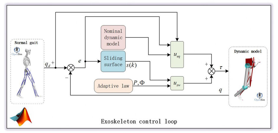
Figure 2. 2-DOF lower limb exoskeleton dynamic simulator block diagram. The exoskeleton controllers are implemented in MATLAB interfacing with the human and exoskeleton models defined in Opensim. 2-DOF: two-degree-of-freedom.

In the following simulation, the established simulation system was run in Matlab software, the simulation time was 3s, the simulation step size was 0.001s, and the standard hip and knee joints of a healthy subject when walking horizontally were used as the reference track.

At the same time, the discrete CSMC algorithm ^[26] and the discrete FTSMC algorithm ^[27] are respectively applied to the dynamics model of the lower limb exoskeleton robot for comparison. The design methods of CSMC and FTSMC are as follows:

1) CSMC

For simplicity, the CSMC ^[26] control input $$ u_{csmc} $$ is given directly:

(49)

$$ \begin{equation} \begin{aligned} u_{csmc} = \left[ {C_{ec}b(k)} \right]^{- 1}\left\lbrack {C_{ec}x_{d}\left( {k + 1} \right) - C_{ec}f(k) - \left( {1 - q_{c}T} \right)s_{c}(k) + \varepsilon_{c}Tsgn\left( s_c(k) \right)} \right\rbrack. \end{aligned} \end{equation} $$

In the formula (49), $$ s_c(k) $$ is the sliding mode variable, which is defined as follows:

(50)

$$ \begin{equation} \begin{aligned} s_{c}(k) = c_{c}e_{c}(k) + {\dot{e}}_{c}(k) \end{aligned} \end{equation} $$

$$ e_c (k) $$ is the tracking error under the control of CSMC, $$ c_{c} = \begin{bmatrix} 15 & 10 \\ \end{bmatrix} $$, $$ \varepsilon_{c} = \begin{bmatrix} 0.01 & 0.01 \\ \end{bmatrix} $$, $$ C_{ec} = \begin{bmatrix} 15 & 0 & 1 & 0 \\ 0 & 10 & 0 & 1 \\ \end{bmatrix} $$.

2) FTSMC

An FTSMC control law ^[27] is also designed for comparison, and the control input $$ u_{ftsmc} $$ is shown below:

(51)

$$ \begin{equation} \begin{aligned} u_{ftsmc}=&[C_{fc}b(k)]^{-1}[C_{fc}(x_{d}(k + 1) - f(k)) -(1 - q_{c}T)s_{f}(k)\\ &+\varepsilon_{c}Tsgn(s(k))-C_{fc2}| s_{f}(k) |^{\alpha}sgn[s_{f}(k)]]. \end{aligned} \end{equation} $$

In Formula (51), $$ s_{f} $$ is a sliding mode variable, defined as follows:

(52)

$$ \begin{equation} \begin{aligned} s_{f}(k) = c{}_{fc1}e_{f}(k) + {\dot{e}}_{f}(k) + C_{fc2}\left| {e_{f}(k)} \right|^{\alpha}sgn\left\lbrack {e_{f}(k)} \right\rbrack \end{aligned} \end{equation} $$

$$ e_f(k) $$ is the tracking error under FTSM control, $$ c_{fc1} = \begin{bmatrix} 15 & 10 \\ \end{bmatrix} $$, $$ c_{fc2} = \begin{bmatrix} 0.05 & 0.05 \\ \end{bmatrix} $$, $$ C_{fc} = \begin{bmatrix} 15 & 0 & 1 & 0 \\ 0 & 10 & 0 & 1 \\ \end{bmatrix} $$.

To test the robustness of the three algorithms to external disturbances, the same external disturbances are set for the three controllers respectively, and the external disturbances are set as:

(53)

$$ \begin{equation} \begin{aligned} {\xi}(k) = \begin{bmatrix} 5sin(k) \\ -5sin(k) \\ \end{bmatrix} (Nm). \end{aligned} \end{equation} $$

The simulation results are shown in Figure 3-6, which are position tracking of the hip joint and knee joint, control input signals, position tracking errors, and sliding mode surface function respectively. In Figure 3, compared with CSMC and FTSMC, the control algorithm proposed in this paper can track the gait trajectory more accurately, and the tracking trajectory of AFOFTSMC is closer to the reference trajectory.

$Human gait tracking for rehabilitation exoskeleton: adaptive fractional order sliding mode control approach$

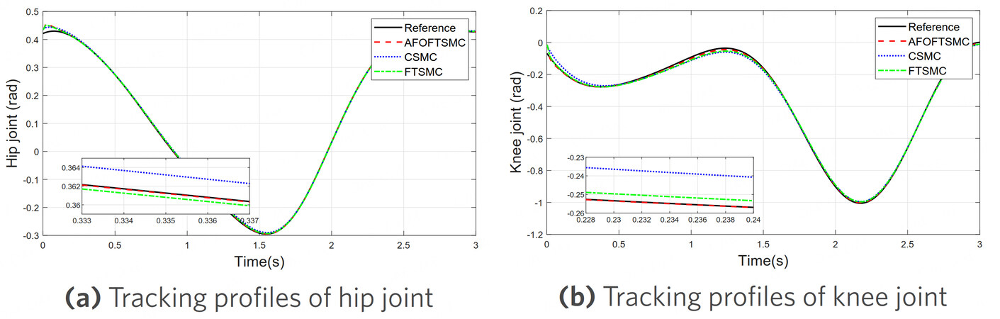
Figure 3. Trajectory tracking performance of the robotic exoskeleton by using CSMC, FTSMC, and AFOFTSMC control strategy. (a) trajectory tracking of the hip joint. (b) trajectory tracking of the knee joint. CSMC: conventional sliding mode control; FTSMC: fast terminal sliding mode control; AFOFTSMC: adaptive fractional order fast terminal sliding mode controller.

$Human gait tracking for rehabilitation exoskeleton: adaptive fractional order sliding mode control approach$

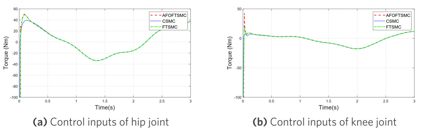
Figure 4. AFOFTSMC control input comparison with CSMC and FTSMC. CSMC: conventional sliding mode control; FTSMC: fast terminal sliding mode control; AFOFTSMC: adaptive fractional order fast terminal sliding mode controller.

$Human gait tracking for rehabilitation exoskeleton: adaptive fractional order sliding mode control approach$

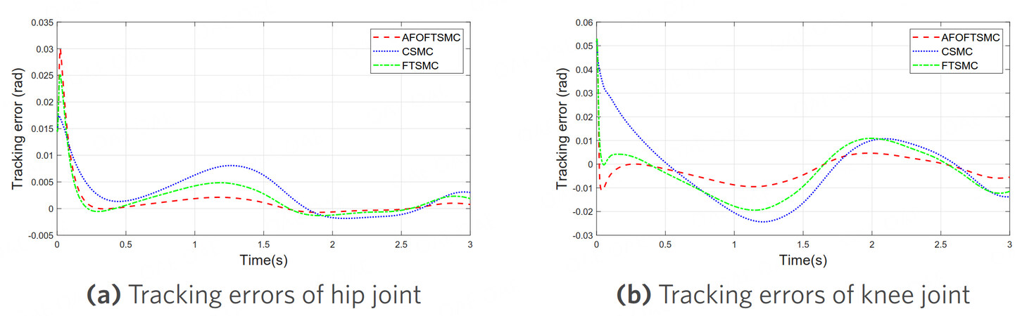
Figure 5. Tracking errors comparison of CSMC, FTSMC, and AFOFTSMC in simulations. (a) errors comparison of the hip joint; (b) errors comparison of the knee joint. CSMC: conventional sliding mode control; FTSMC: fast terminal sliding mode control; AFOFTSMC: adaptive fractional order fast terminal sliding mode controller.

$Human gait tracking for rehabilitation exoskeleton: adaptive fractional order sliding mode control approach$

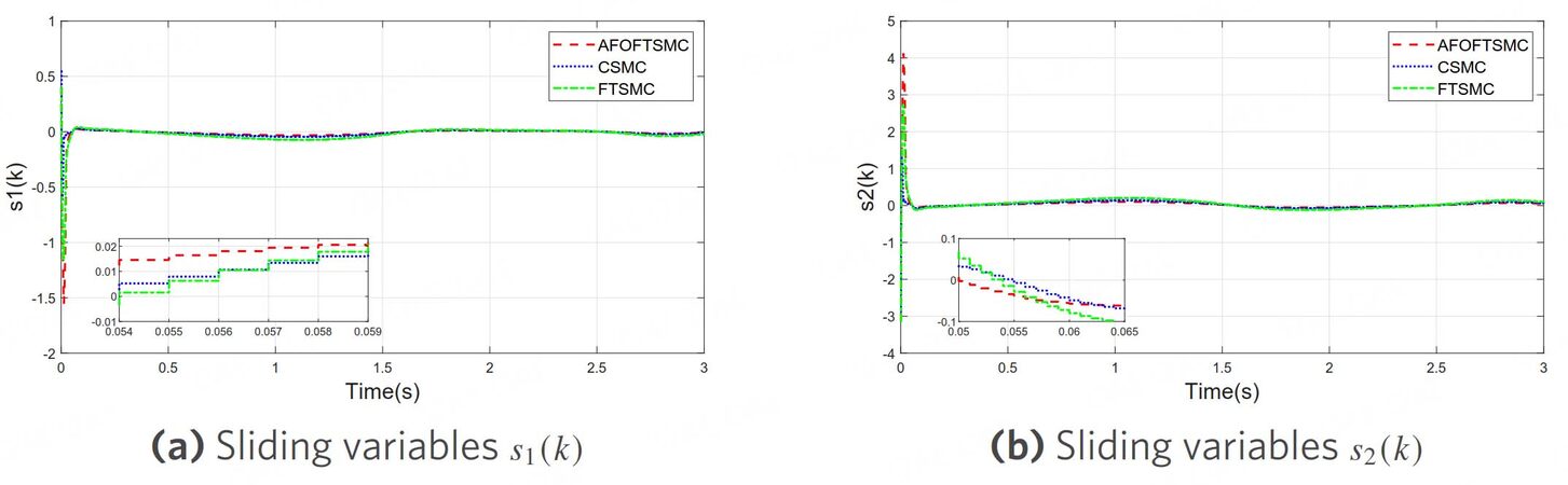
Figure 6. Sliding variables for the three sliding surfaces.

Moreover, it can be seen from Figure 4 that the control inputs of AFOFTSMC do not need to give greater control efforts to maintain higher track tracking accuracy and effectively eliminate the impact of external interference. According to the comparison of tracking errors in Figure 5, the AFOFTSMC algorithm has the smallest steady-state tracking error, which can ensure that the system error converges in a finite time. In Figure 6, the sliding mode variables of the three controllers can move rapidly into the quasi-sliding mode band, and the control algorithm proposed in this paper can effectively reduce the width of the quasi-sliding mode band.

To provide more quantitative proof, three indicators are compared in Table 1 to evaluate the performance of three different control strategies. Mean absolute error (MAE) with $$ MAE=\frac{1}{N}\sum_{k=1}^{N}{|e(k)|} $$, maximum tracking error (MTE) with $$ MTE=max|e(k)| $$, root mean square error (RMSE) with $$ RMSE=\sqrt{\frac{1}{N}\sum_{k=1}^{N}{[e(k)]^2}} $$. The results are shown in Table 1. The discrete adaptive fractional order fast terminal sliding mode control algorithm proposed in this paper is applied to the lower limb exoskeleton robot to achieve better trajectory tracking control. The generated RMSE and MAE are both minima, but the MTE is maximum, which is due to overdrive caused by fast response speed.

Table 1

Performance indicators of the three controllers

Controllers	RMSE of hip	MAE of hip	MTE of hip	RMSE of knee	MAE of knee	MTE of knee
AFOFTSMC (Proposed)	0.0056 rad	0.0026 rad	0.0300 rad	0.0075 rad	0.0057 rad	0.0529 rad
CSMC ^[26]	0.0066 rad	0.0056 rad	0.0174 rad	0.0189 rad	0.0166 rad	0.0529 rad
FTSMC ^[27]	0.0056 rad	0.0370 rad	0.0253 rad	0.0128 rad	0.0105 rad	0.0529 rad

To enhance SMC's ability to resist external disturbances, we use fractional order sliding mode surfaces to accelerate the convergence of system errors and make adaptive adjustments to control law parameters. Compared with the traditional control methods, AFOFTSMC has better potential to be applied to the actual exoskeleton rehabilitation robot and help patients to carry out rehabilitation training in the early stage of rehabilitation. In addition to the field of rehabilitation robots, the algorithm can also be extended to other fields to achieve better control effects, such as chaotic systems, robot manipulators, and quadrotor UAVs.

5. CONCLUSIONS

In this paper, we study a human gait trajectory-tracking control issue of lower limb exoskeleton rehabilitation robot. Firstly, the dynamic properties of the lower limb exoskeleton rehabilitation robot were analyzed. Then, a new AFOFTSMC algorithm was developed for the lower limb exoskeleton robot with uncertain parameters and unknown external interference, where the fractional order fast terminal sliding mode function was introduced to achieve rapid convergence in finite time. Particularly, the unknown dynamic part of the exoskeleton was processed by adaptive law, and the width of the quasi-sliding mode band was adjusted in real-time to ensure that the sliding mode variables quickly enter the quasi-sliding mode band. Moreover, the stability of the whole control system was verified in the Lyapunov sense. To illustrate the effectiveness of the proposed controller, we compared the simulation results of CSCM, FTSMC, and AFOFTSMC on the MATLAB-Opensim co-simulation platform. The simulation results showed that the adaptive fractional order fast terminal sliding mode controller has the characteristics of high precision, fast response, and strong robustness for robot trajectory tracking.

DECLARATIONS

Authors' contributions

Implemented the methodologies presented and wrote the paper: Zhou Y, Sun Z

Performed oversight and leadership responsibility for the research activity planning and execution, as well as developed ideas and evolution of overarching research aims: Sun Z, Chen B, Wang T

Performed critical review, commentary, and revision, as well as providing technical guidance: Sun Z, Chen B, Wu X, Huang G

All authors have revised the text and agreed to the published version of the manuscript.

Availability of data and materials

Not applicable.

Financial support and sponsorship

This work was supported by the Primary Research and Development Plan of Zhejiang Province (No. 2022C03029)

Conflicts of interest

All authors declared that there are no conflicts of interest.

Ethical approval and consent to participate

Not applicable.

Consent for publication

Not applicable.

Copyright

REFERENCES

1. Liu WL, Yin BL, Yan BB. A survey on the exoskeleton rehabilitation robot for the lower limbs. In: 2016 2nd International Conference on Control, Automation and Robotics (ICCAR); 2016 Apr 28-30; Hong Kong, China. IEEE; 2016. pp. 90–94.

2. Meng W, Liu Q, Zhou ZD, Ai QS, Sheng B, Xie SQ. Recent development of mechanisms and control strategies for robot-assisted lower limb rehabilitation. Mechatronics 2015;31:132-45.

3. Han J, Yang SY, Xia L, Chen YH. Deterministic adaptive robust control with a novel optimal gain design approach for a fuzzy 2-DOF lower limb exoskeleton robot system. IEEE Trans Fuzzy Syst 2021;29:2373-87.

4. Sun W, Lin JW, Su SF, Wang N, Er MJ. Reduced adaptive fuzzy decoupling control for lower limb exoskeleton. IEEE Trans Cybern 2021;51:1099-109.

5. Long Y, Du ZJ, Cong L, Wang WD, Zhang ZM, Dong W. Active disturbance rejection control based human gait tracking for lower extremity rehabilitation exoskeleton. ISA Trans 2017;67:389-97.

6. Asl HJ, Narikiyo T, Kawanishi M. Neural network-based bounded control of robotic exoskeletons without velocity measurements. Contr Eng Pract 2018;80:94-104.

7. Torres FJ, Guerrero GV, García CD, Gomez JF, Adam M and Escobar RF. Master-slave synchronization of robot manipulators driven by induction motors. IEEE Latin Am Trans 2016;14:3986-91.

8. Ahmed S, Wang HP, Tian Y. Robust adaptive fractional-order terminal sliding mode control for lower-limb exoskeleton. Asian J of Contr 2019;21:473-82.

9. Narayan J, Abbas M, Patel B, Dwivedy SK. A Singularity-free terminal sliding mode control of an uncertain paediatric exoskeleton system. In: 2022 5th International Conference on Advanced Systems and Emergent Technologies (IC_ASET); 2022 Mar 22-25; Hammamet, Tunisia. IEEE; 2022. pp. 198–203.

10. Cao SB, Cao GZ, Zhang YP, Ling ZQ, He BB, Huang SD. Fast-terminal sliding mode control based on dynamic boundary layer for lower limb exoskeleton rehabilitation robot. In: 2021 IEEE 11th Annual International Conference on CYBER Technology in Automation, Control, and Intelligent Systems (CYBER); 2021 July 27-31; Jiaxing, China. IEEE; 2021. pp. 453–458.

11. Chen SB, Beigi A, Yousefpour A, et al. Recurrent neural network-based robust nonsingular sliding mode control with input saturation for a non-holonomic spherical robot. IEEE Access 2020;8:188441-53.

12. Fei JT, Feng ZL. Fractional-order finite-time super-twisting sliding mode control of micro gyroscope based on double-loop fuzzy neural network. IEEE Trans Syst Man Cybern, Syst 2021;51:7692-706.

13. Wang YY, Gu LY, Xu YH, Cao XX. Practical tracking control of robot manipulators with continuous fractional-order nonsingular terminal sliding mode. IEEE Trans Ind Electron 2016;63:6194-204.

14. Yang Y, Chen YQ, Chu YZ, Wang Y, Liang Q. Fractional order adaptive sliding mode controller for permanent magnet synchronous motor. In: 2016 35th Chinese Control Conference (CCC); 2016 July 27-29; Chengdu, China. IEEE; 2016. pp. 3412–3416.

15. Lavín-Delgado JE, Chávez-Vázquez S, Gómez-Aguilar JF, Alassafi MO, Alsaadi FE, Ahmad AM. Intelligent Neural Integral Sliding-mode Controller for a space robotic manipulator mounted on a free-floating satellite. Adv Space Res 2022; Epub ahead of print.

16. Lavín-Delgado JE, Beltrán ZZ, Gómez-Aguilar JF, Pérez-Careta E. Controlling a quadrotor UAV by means of a fractional nested saturation control. Adv Space Res 2022; Epub ahead of print.

17. Li JF, Jahanshahi H, Kacar S, et al. On the variable-order fractional memristor oscillator: Data security applications and synchronization using a type-2 fuzzy disturbance observer-based robust control. Chaos, Solitons & Fractals 2021;145:110681.

18. Wang YL, Jahanshahi H, Bekiros S, Bezzina F, Chu YM, Aly AA. Deep recurrent neural networks with finite-time terminal sliding mode control for a chaotic fractional-order financial system with market confidence. Chaos, Solitons & Fractals 2021;146:110881.

19. Xiong PY, Jahanshahi H, Alcaraz R, Chu YM, Gómez-Aguilar JF, Alsaadi FE. Spectral entropy analysis and synchronization of a multi-stable fractional-order chaotic system using a novel neural network-based chattering-free sliding mode technique. Chaos, Solitons & Fractals 2021;144:110576.

20. Li SH, Du HB, Yu XH. Discrete-time terminal sliding mode control systems based on euler's discretization. IEEE Trans Automat Contr 2014;59:546-52.

21. Chen B, Hu GQ, Ho DWC, Yu L. Distributed Estimation and Control for Discrete Time-Varying Interconnected Systems. IEEE Trans Automat Contr 2022;67:2192-207.

22. Sun GH, Ma ZQ, Yu JY. Discrete-time fractional order terminal sliding mode tracking control for linear motor. IEEE Trans Ind Electron 2018;65:3386-94.

23. Ajjanaromvat N, Parnichkun M. Trajectory tracking using online learning LQR with adaptive learning control of a leg-exoskeleton for disorder gait rehabilitation. Mechatronics 2018;51:85-96.

24. Neuman CP, Tourassis VD. Discrete dynamic robot models. IEEE Trans Syst, Man, Cybern 1985;SMC-15:193-204.

25. Zhou Y, Hu ZY, Sun Z, Wang T, Chen B. Covariance intersection fusion approach for gait estimation of lower limb rehabilitation Exoskeleton Robot. In: 2022 5th International Symposium on Autonomous Systems (ISAS); 2022 April 08-10; Hangzhou, China. IEEE; 2022. pp. 1–6.

26. Gao WB, Wang YF, A HMF. Discrete-time variable structure control systems. IEEE Trans Ind Electron 1995;42:117-22.

27. Wang Z, Li SH, Li Q. Discrete-time fast terminal sliding mode control design for DC-DC buck converters with mismatched disturbances. IEEE Trans Ind Inf 2020;16:1204-13.

28. Delp SL, Anderson FC, Arnold AS, et al. OpenSim: open-source software to create and analyze dynamic simulations of movement. IEEE Trans Biomed Eng 2007;54:1940-50.

29. Seth A, Hicks JL, Uchida TK, et al. OpenSim: Simulating musculoskeletal dynamics and neuromuscular control to study human and animal movement. PLoS Comput Biol 2018;14:e1006223.

30. Mi WM, Zhang T. Fuzzy variable impedance adaptive robust control algorithm of exoskeleton robots. In: 2019 Chinese Control Conference (CCC); 2019 July 27-30; Guangzhou, China. IEEE; 2019. pp. 4302–7.

Cite This Article

Export citation file: BibTeX | RIS

OAE Style

Zhou Y, Sun Z, Chen B, Huang G, Wu X, Wang T. Human gait tracking for rehabilitation exoskeleton: adaptive fractional order sliding mode control approach. Intell Robot 2023;3(1):95-112. http://dx.doi.org/10.20517/ir.2023.05

AMA Style

Zhou Y, Sun Z, Chen B, Huang G, Wu X, Wang T. Human gait tracking for rehabilitation exoskeleton: adaptive fractional order sliding mode control approach. Intelligence & Robotics. 2023; 3(1): 95-112. http://dx.doi.org/10.20517/ir.2023.05

Chicago/Turabian Style

Zhou, Yuan, Zhe Sun, Bo Chen, Guangpu Huang, Xiang Wu, Tian Wang. 2023. "Human gait tracking for rehabilitation exoskeleton: adaptive fractional order sliding mode control approach" Intelligence & Robotics. 3, no.1: 95-112. http://dx.doi.org/10.20517/ir.2023.05

ACS Style

Zhou, Y.; Sun Z.; Chen B.; Huang G.; Wu X.; Wang T. Human gait tracking for rehabilitation exoskeleton: adaptive fractional order sliding mode control approach. Intell. Robot. 2023, 3, 95-112. http://dx.doi.org/10.20517/ir.2023.05

About This Article

Special Issue

This article belongs to the Special Issue Advances in Human-Assistive Technologies and Human-Robot Interactions

Copyright

© The Author(s) 2023. Open Access This article is licensed under a Creative Commons Attribution 4.0 International License (https://creativecommons.org/licenses/by/4.0/), which permits unrestricted use, sharing, adaptation, distribution and reproduction in any medium or format, for any purpose, even commercially, as long as you give appropriate credit to the original author(s) and the source, provide a link to the Creative Commons license, and indicate if changes were made.

Data & Comments

Data

Views

599

Downloads

500

Citations

Comments

Comments

Comments must be written in English. Spam, offensive content, impersonation, and private information will not be permitted. If any comment is reported and identified as inappropriate content by OAE staff, the comment will be removed without notice. If you have any queries or need any help, please contact us at support@oaepublish.com.