Research Article | Open Access | 26 Jun 2023

Adaptive backstepping control of high-order fully actuated nonlinear systems with event-triggered strategy

Views: 427 | Downloads: 55 | Cited:

Chengyuan Yan

, ...

Chong Li

Intell Robot 2023;3(2):176-89.

10.20517/ir.2023.11 | © The Author(s) 2023.

Author Information

Article Notes

Cite This Article

Abstract

This paper investigates the problem of adaptive event-triggered fuzzy control for nonlinear high-order fully actuated systems. In this paper, a completely unknown nonlinear function is considered, and its prior knowledge is unknown. To solve this problem, the fuzzy logic system technology is applied to approximate the unknown nonlinear function. In order to save communication resources, a novel high-order event-triggered controller is proposed under backstepping control. With the help of Lyapunov stability theory, it is proved that all signals of the closed-loop system are bounded. Finally, the theoretical results are applied to the robot system to verify their validity.

Keywords

fuzzy logic system, event-triggered strategy, high-order fully actuated nonlinear systems, adaptive control

Download PDF 0 4

1. INTRODUCTION

With the development of modern society and modern industry, linear system theory has become relatively well-established and sophisticated^[1–3]. Many scholars have proposed various powerful analysis tools for linear systems. However, with the progress of science and technology and the improvement of the accuracy of measuring tools, the understanding of the actual system is gradually deepened, and the requirements for its control performance are also increasingly high. Ignoring some objective factors, some practical systems are modeled as linear systems and controller designs are carried out, but the designed controllers have not met the requirements for the control performance of practical systems. In such cases, it is particularly necessary to model some practical systems into nonlinear systems. This includes systems such as unmanned vehicle systems^[4], unmanned aerial vehicle systems^[5], robot systems, and manipulator systems^[6]. Therefore, nonlinear systems have received extensive attention from scholars at home and abroad and have proposed various tools to handle the control problem of nonlinear systems, such as adaptive backstepping control^{[7, 8]}, sliding mode control^[9], etc. Among them, the combination of backstepping recursive design and adaptive control has produced a large number of excellent results^[10–14].

The high-order fully actuated system possesses unparalleled control characteristics compared to other systems. Its fully actuated characteristics enable the elimination of all dynamic characteristics of the open-loop system while establishing new and desired closed-loop dynamic characteristics. About high-order fully actuated systems, there have been some excellent results^[15–23]. Among them, The work^[19] proposed the direct parametric approach of fully-actuated high-order systems. A constrained cooperative control is proposed^[22] for high-order fully actuated multiagent systems with prescribed performance.

Since the beginning of this century, networked control systems^[24–29] have been widely used in remote operation, industrial automation, building energy conservation, and other fields. This is due to their low maintenance cost and high flexibility. In the networked control system, the actuator, controller, sensor, and other components transmit information through the shared network channel. Therefore, it is necessary to reduce the occupation of shared communication by single subsystem control to achieve the purpose of saving cost and energy. The traditional sampling control^[30–33] is based on the system signal sampling value instead of continuous value and takes different constant values periodically, which has relatively high communication efficiency compared with continuous time control. Sampling control requires information transmission and control update at a conservative fixed frequency regardless of obvious changes in system performance, so it is not suitable for networked control systems with high integration, which leads to the emergence of more efficient control of resource utilization, namely event-triggered control. The key point of the event-triggered control design is to build an event-triggered mechanism. The most basic types are absolute threshold type, relative threshold type, and mixed threshold type. The construction of an event-triggered mechanism depends not only on the system structure but also on the expected control objectives. Even with the increase in system complexity and performance requirements, additional dynamic and online adjustment parameters need to be introduced. Over the past decade, significant progress has been made in the research of event-triggered control for nonlinear systems^[34–43].

Inspired by the above excellent results and combined with the reality of the lack of event-triggered control results of the high-order fully activated system, this paper studies the adaptive fuzzy event-triggered control for the high-order fully activated system. The contribution of this paper is reflected in two aspects:

1) For the uncertain high-order fully actuated nonlinear system, the unknown nonlinear function is considered, and the fuzzy logic system (FLS) is used to approximate the nonlinear function without a priori condition of the nonlinear function.

2) The proposed event-triggered scheme for the uncertain high-order fully nonlinear system can effectively eliminate the continuous update of the designed controller, thus saving communication resources.

The organization of this article is arranged as follows. The second section includes problem formulas and preliminary knowledge. The third section introduces an event-triggered controller design scheme. The fourth section shows the simulation. The fifth section is the summary.

Notation

$$ I_n $$ represents the identity matrix and

$$ {x^{(0\sim n)}}= \begin{bmatrix} x \\ \dot{x} \\ \vdots \\ x^{(n)} \end{bmatrix} , $$

$$ {A^{0\sim n-1}}= \begin{bmatrix} A_0 &A_1&\ldots&A_{n-1} \end{bmatrix} , $$

$$ {I^{\circ}_n}= \begin{bmatrix} 0& 0 &1 \\ 0 & \ddots & 0 \\ 1 & 0 & 0 \end{bmatrix} , $$

$$ {x^{(0\sim n)}_{i\sim j}}= \begin{bmatrix} x_i^{(0\sim n)} \\ x_{i+1}^{(0\sim n)} \\ \vdots \\ x_{j}^{(0\sim n)} \end{bmatrix} , j\geq i $$

$$ {\Phi(A^{0\sim n-1})}= \begin{bmatrix} 0& I & & \\ & & \ddots& \\ & & &I\\ -A_0 &-A_1&\ldots&A_{n-1} \end{bmatrix} . $$

2. PROBLEM FORMULAS AND PRELIMINARY KNOWLEDGE

2.1. Problem statement

Consider the following uncertain high-order fully nonlinear system:

(1)

$$ \begin{equation} \left\{ \begin{aligned} {x}^{(p_1)}_1 =&g_1(x_{1}^{(0\sim p_1-1)})x_2+f_1(x_{1}^{(0\sim p_1-1)}), \\ {x}^{(p_j)}_j =& g_j(x_{i}^{(0\sim p_i-1)}|_{i=1\sim j})x_{j+1}+f_j(x_{i}^{(0\sim p_i-1)}|_{i=1\sim j}), \\ {x}^{(p_n)}_n =& g_n(x_{i}^{(0\sim p_i-1)}|_{i=1\sim n})u+f_n(x_{i}^{(0\sim p_i-1)}|_{i=1\sim n}), \end{aligned} \right. \end{equation} $$

where $$ p_i\in\mathbb{N}^{+} $$, and $$ u $$ denotes the system input. $$ f_i(x_{i}^{(0\sim p_i-1)}|_{i=1\sim j}) $$ are sufficiently smooth unknown nonlinear functions, $$ g_i(x_{i}^{(0\sim p_i-1)}|_{i=1\sim j}) $$ are control gain functions, and satisfy full-actuation conditions.

Remark 1The above-mentioned high-order fully nonlinear system is the general form of a second-order fully nonlinear system. For practical examples, such as robotic systems, it is no longer necessary to transform a high-order system into a first-order system. Instead, we can deal with it directly.

2.2. Preliminaries knowledge

Assumption 1^[37] There are two constants that the control gain functions $$ 0<\underline{g}_j\leq|g_j(x_{i}^{(0\sim p_i\!-\!1)}|_{i=1\sim j})|\leq \bar{g}_j, j=1, \cdots, n $$.

Remark 2The above assumption is a common standard condition that ensures the controllability of the uncertain high-order fully nonlinear system. This is derived from modeling real systems, and it makes perfect sense.

Lemma 1^[38] The unknown nonlinear continuous function $$ \zeta(\xi) $$ is defined on a compact set. And there is an FLS satisfying the following inequality

(2)

$$ \zeta(\xi)=W^{*T}S(\xi)+\delta(\xi), $$

where $$ \delta(\xi) $$ indicates the any estimation error which satisfies $$ |\delta(x)|\leq\overline{\delta} $$.

Lemma 2^[38] For $$ \forall\epsilon>0 $$ and $$ \sigma\in{R} $$, it can be concluded that

(3)

$$ 0\leq|\sigma|-\sigma\tanh(\frac{\sigma}{\epsilon})\leq0.2785\epsilon. $$

Lemma 3^[18] Design the matrix $$ A_i^{0\sim p_i-1}\in \mathbb{R}^{1\times p_i} $$ so that the matrix $$ \Phi(A_i^{0\sim p_i-1})\in \mathbb{R}^{p_i\times p_i} $$ is stable. Moreover, according to Lyapunov Theorem, there is a matrix $$ P_i(A_i^{0\sim p_i-1})\in \mathbb{R}^{p_i\times p_i} $$, which is positive definite, satisfying

(4)

$$ \Phi{(A_i^{0\sim p_i-1})}^T\!P_i(A_i^{0\sim p_i-1})\!+\!P_i(A_i^{0\sim p_i-1})\Phi{(A_i^{0\sim p_i-1})} =-\rho_i I_i, $$

where $$ \rho_i>0 $$ ($$ i=1, \cdots, n $$) are design parameters.

3. CONTROLLER DESIGN AND STABILITY ANALYSIS

3.1. Adaptive event-triggered controller design

To facilitate the calculation, we first give some necessary coordinate transformations:

$$ \tilde{P}_i(A_i^{0\sim p_i-1})=I^\circ_2P_i^T(A_i^{0\sim p_i-1}) , $$

$$ P_i(A_i^{0\sim p_i-1})= \begin{bmatrix} P_{iF}(A_i^{0\sim p_i-1})&\cdots &P_{iL}(A_i^{0\sim p_i-1}) \end{bmatrix} , $$

$$ \tilde{P}^{-1}_i(A_i^{0\sim p_i-1}) = \begin{bmatrix} Q_{i11}(A_i^{ 0\sim p_i-1}) & Q_{i12}(A_i^{ 0\sim p_i-1}) & Q_{i13}(A_i^{ 0\sim p_i-1})\\ Q_{iF}(A_i^{ 0\sim p_i-1}) & Q_{iM}(A_i^{ 0\sim p_i-1}) & Q_{iL}(A_i^{ 0\sim p_i-1}) \end{bmatrix} , $$

where $$ Q_{iL}(A_i^{0\sim p_i-1})\neq0 $$ ($$ i=1, \cdots, n $$).

Step 1: Let

(5)

$$ \ \ \ s_1^{(0\sim p_1-1)}=x_1^{(0\sim p_1-1)}, $$

and

$$ \tilde{P}_2(A_2^{0\sim p_2-1})s_2^{(0\sim p_2-1)}=x_2^{(0\sim p_2-1)}- \begin{bmatrix} \alpha_1 \\ 0 \end{bmatrix} . $$

With the help of the notations, one has

$$ P_{2L}^T(A_2^{0\sim p_2-1})s_2^{(0\sim p_2-1)} =x_2-\alpha_1. $$

Choose virtual controller $$ \alpha_1 $$ as

(6)

$$ \alpha_1= -\frac{1}{g_1(x_{1}^{(0\sim p_1-1)})}(A_1^{(0\sim p_1-1)}s_1^{(0\sim p_1-1)} +\frac{1}{2a_1^2}P_{1L}^T(A_1^{0\sim p_1-1})s_1^{(0\sim p_1-1)}\hat{\theta}_1S_1^TS_1 +\frac{1}{2}P_{1L}^T(A_1^{0\sim p_1-1})s_1^{(0\sim p_1-1)}). $$

The Lyapunov candidate function $$ V_{1} $$ is designed as

(7)

$$ V_{1}=(s_1^{(0\sim p_1-1)})^T P_1(A_1^{0\sim p_1-1})s_1^{(0\sim p_1-1)}+\frac{1}{2}\tilde{\theta}_1^2, $$

where $$ \theta_1=\max\{\|W_1\|^2\} $$, $$ \tilde{\theta}_1=\theta_1-\hat{\theta}_1 $$, and $$ \hat{\theta}_1 $$ is the estimation of $$ \theta_1 $$.

With the help of FLS and Young's inequality, one gets

(8)

$$ \begin{align} &P_{1L}^T(A_1^{0\sim p_1-1})s_1^{(0\sim p_1-1)}F_1(X_{1}) =P_{1L}^T(A_1^{0\sim p_1-1})s_1^{(0\sim p_1-1)}(W_1^TS_1(X_1)+\delta_1)\\ \leq&\frac{(P_{1L}^T(A_1^{0\sim p_1-1})s_1^{(0\sim p_1-1)})^2\theta_1S_1^T(X_1)S _1(X_1)}{2a_1^2}+\frac{1}{2}a_1^2 +\frac{1}{2}P_{1L}^T(A_1^{0\sim p_1-1})s_1^{(0\sim p_1-1)}P_{1L}^T(A_1^{0\sim p_1-1})s_1^{(0\sim p_1-1)}\!+\!\frac{1}{2}\bar{\delta}_1^2, \end{align} $$

where $$ F_1(X_1)=f_1(x_{1}^{(0\sim p_1-1)}) $$, $$ X_1=[x_1^{(0\sim p_1-1)}] $$ and $$ a_1 $$ is a constant.

The adaptive law $$ \hat{\theta}_1 $$ is chosen as

(9)

$$ \dot{\hat{\theta}}_1= \frac{1}{a_1^2}P_{1L}^T(A_1^{0\sim p_1-1})s_1^{(0\sim p_1-1)} P_{1L}^T(A_1^{0\sim p_1-1})s_1^{(0\sim p_1-1)}S_1^TS_1-l_1\hat{\theta}_1. $$

Based on (8) and (9), one gets

(10)

$$ \begin{align} \dot{V}_{1}\leq&-\rho_1(s_1^{(0\sim p_1-1)})^Ts_1^{(0\sim p_1-1)}-\frac{1}{2}l_1\tilde{\theta}_1^2+a_1^2+\bar{\delta}_1^2+\frac{1}{2}l_1\theta_1^2\\ &+2P_{1L}^T(A_1^{0\sim p_1-1})s_1^{(0\sim p_1-1)}g_1(x_{1}^{(0\sim p_1-1)}) P_{2L}^T(A_2^{0\sim p_2-1})s_2^{(0\sim p_2-1)}. \end{align} $$

Step 2: Based on the notations, one has

(11)

$$ P_{3L}^T(A_3^{0\sim p_3-1})s_3^{(0\sim p_3-1)} =x_3-\alpha_2, $$

From (1) and (11), the time derivative of $$ s_2 $$ is

(12)

$$ \begin{align} s_2^{(p_2)}=&Q_{2F}(A_2^{0\sim p_2-1})(\dot{x}_2-\dot{\alpha}_1)+Q_{2M}(A_2^{0\sim p_2-1})\dot{x}_2^{(1\sim p_2-2)} +Q_{2L}(A_2^{0\sim p_2-1})f_2(x_{i}^{(0\sim p_i-1)}|_{i=1\sim 2})\\ &+Q_{2L}(A_2^{0\sim p_2-1})g_2(x_{i}^{(0\sim p_i-1)}|_{i=1\sim 2}) P_{3L}(A_3^{(0\sim p_3-1)})s_3^{(0\sim p_3-1)} +Q_{2L}(A_2^{0\sim p_2-1})g_2(x_{i}^{(0\sim p_i-1)}|_{i=1\sim 2})\alpha_2. \end{align} $$

Choose virtual controller $$ \alpha_2 $$ as

(13)

$$ \begin{align} \alpha_2=&-\frac{1}{Q_{2L}(A_2^{0\sim p_2-1})g_2(x_{i}^{(0\sim p_i\!-\!1)}|_{i=1\sim 2})}(A_2^{(0\sim p_2-1)} s_2^{(0\sim p_2\!-\!1)}\\ &+\frac{1}{2a_2^2}P_{2L}^T(A_2^{0\sim p_2-1})s_2^{(0\sim p_2-1)} \hat{\theta}_2S_2^TS_2 +\frac{1}{2}P_{2L}^T(A_2^{0\sim p_2-1})s_2^{(0\sim p_2-1)}), \end{align} $$

and (12) can be rewritten as state-space form

$$ \dot{s}_2^{(0\sim p_2-1)}={\Phi(A_2^{0\sim p_2-1})}s_2^{(0\sim p_2-1)}+ \begin{bmatrix} 0 \\ H_2 \end{bmatrix} $$

where

$$ H_2=Q_{2F}(A_2^{0\sim p_2-1})(\dot{x}_2\!-\!\dot{\alpha}_1)\!-\!\frac{1}{2a_2^2}P_{2L}^T(A_2^{0\sim p_2-1})s_2^{(0\sim p_2-1)} \hat{\theta}_2S_2^TS_2+Q_{2M}(A_2^{0\sim p_2-1})\dot{x}_2^{(1\sim p_2-2)}+Q_{2L}(A_2^{0\sim p_2-1})$$$$ \times f_2(x_{i}^{(0\sim p_i-1)}|_{i=1\sim 2}) -\frac{1}{2}P_{2L}^T(A_2^{0\sim p_2-1})s_2^{(0\sim p_2-1)}) +Q_{2L}(A_2^{0\sim p_2-1}) g_2(x_{i}^{(0\sim p_i-1)}|_{i=1\sim 2})P_{3L}(A_3^{(0\sim p_3-1)})s_3^{(0\sim p_3-1)} $$.

The Lyapunov function candidate $$ V_{2} $$ is presented as

(14)

$$ V_{2}=V_{1}+(s_2^{(0\sim p_2-1)})^T P_2(A_2^{0\sim p_2-1})s_2^{(0\sim p_2-1)}+\frac{1}{2}\tilde{\theta}_2^2. $$

And similar to the (8), one gets

(15)

$$ \begin{align} &P_{2L}^T(A_2^{0\sim p_2-1})s_2^{(0\sim p_2-1)}F_2(X_{2}) =P_{2L}^T(A_2^{0\sim p_2-1})s_2^{(0\sim p_2-1)}(W_2^TS_2(X_2)+\delta_2)\\ \leq&\frac{(P_{2L}^T(A_2^{0\sim p_2-1})s_2^{(0\sim p_2-1)})^2\theta_2S_2^T(X_2)S _2(X_2)}{2a_2^2}+\frac{1}{2}a_2^2 +\frac{1}{2}P_{2L}^T(A_2^{0\sim p_2-1})s_2^{(0\sim p_2-1)}P_{2L}^T(A_2^{0\sim p_2-1})s_2^{(0\sim p_2-1)}+\frac{1}{2}\bar{\delta}_2^2 \end{align} $$

where

$$ F_{2}(X_{2})=Q_{2F}(A_2^{0\sim p_2-1})(\dot{x}_2-\dot{\alpha}_1)+Q_{2M}(A_2^{0\sim p_2-1})\dot{x}_2^{(1\sim p_2-2)}+Q_{2L}(A_2^{0\sim p_2-1})f_2(x_{i}^{(0\sim p_i-1)}|_{i=1\sim 2}) +P_{1L}^T(A_1^{0\sim p_1-1})s_1^{(0\sim p_1-1)} $$, $$ X_2=[x_1^{(0\sim p_1-1)}, x_2^{(0\sim p_2-1)}, \hat{\theta}_1] $$.

The adaptive update law $$ \hat{\theta}_2 $$ is designed as

(16)

$$ \dot{\hat{\theta}}_2= \frac{1}{a_2^2}P_{2L}^T(A_2^{0\sim p_2-1})s_2^{(0\sim p_2-1)} P_{2L}^T(A_2^{0\sim p_2-1})s_2^{(0\sim p_2-1)}S_2^TS_2-l_2\hat{\theta}_2. $$

Replacing (15) and (16) into (14), one gives

(17)

$$ \begin{align} \dot{V}_{2}\leq&-\sum\limits_{j=1}^{2}\tau_j(s_j^{(0\sim p_j-1)}|_{j=1\sim 2})^T(s_j^{(0\sim p_j-1)}|_{j=1\sim 2})+\sum\limits_{j=1}^{2}(a_j^2 +\bar{\delta}_j^2+\frac{1}{2}l_j\theta_j^2)-\sum\limits_{j=1}^{2}\frac{l_j}{2}\tilde{\theta}_j^2\\ &+2P_{2L}^T(A_2^{0\sim p_2-1})s_2^{(0\sim p_2-1)}Q_{2L}(A_2^{0\sim p_2-1}) g_2(x_{i}^{(0\sim p_i-1)}|_{i=1\sim 2})P_{3L}(A_3^{(0\sim p_3-1)})s_3^{(0\sim p_3-1)} \end{align} $$

Step k:$$ (3\leq k \leq n-1) $$ Based on the notations, one has

(18)

$$ P_{kL}^T(A_k^{0\sim p_k-1})s_k^{(0\sim p_k-1)} =x_k-\alpha_{k-1}, $$

Choose virtual controller $$ \alpha_k $$ as

(19)

$$ \begin{align} \alpha_k=&-\frac{1}{Q_{kL}(A_k^{0\sim p_k-1})g_k(x_{i}^{(0\sim p_i-1)}|_{i=1\sim k})}(A_k^{(0\sim p_k-1)} s_k^{(0\sim p_k-1)}\\ &+\frac{1}{2a_k^2}P_{kL}^T(A_k^{0\sim p_k-1})s_k^{(0\sim p_k-1)} \hat{\theta}_kS_k^TS_k +\frac{1}{2}P_{kL}^T(A_k^{0\sim p_k-1})s_k^{(0\sim p_k-1)}). \end{align} $$

The Lyapunov function candidate $$ V_{k} $$ is presented as

(20)

$$ V_{k}=V_{k-1}+(s_k^{(0\sim p_k-1)})^T P_k(A_k^{0\sim p_k-1})s_k^{(0\sim p_k-1)}+\frac{1}{2}\tilde{\theta}_k^2. $$

And similar to the (8), one gets

(21)

$$ \begin{align} &P_{kL}^T(A_k^{0\sim p_k-1})s_k^{(0\sim p_k-1)}F_k(X_{k}) =P_{kL}^T(A_k^{0\sim p_k-1})s_k^{(0\sim p_k-1)}(W_k^TS_k(X_k)+\delta_k)\\ \leq&\frac{(P_{kL}^T(A_k^{0\sim p_k-1})s_k^{(0\sim p_k-1)})^2\theta_kS_k^T(X_k)S _k(X_k)}{2a_k^2}+\frac{1}{2}a_k^2 +\frac{1}{2}P_{kL}^T(A_k^{0\sim p_k-1})s_k^{(0\sim p_k-1)}P_{kL}^T(A_k^{0\sim p_k-1})s_k^{(0\sim p_k-1)}+\frac{1}{2}\bar{\delta}_k^2 \end{align} $$

where

$$ F_{k}(X_{k})=Q_{kF}(A_k^{0\sim p_k-1})(\dot{x}_k\!-\!\dot{\alpha}_{k-1})+Q_{kM}(A_k^{0\sim p_k-1})\dot{x}_k^{(1\sim p_k-2)}+Q_{kL}(A_k^{0\sim p_k-1})f_k(x_{i}^{(0\sim p_i-1)}|_{i=1\sim k})$$

$$ +P_{kL}^T(A_k^{0\sim p_k-1})s_k^{(0\sim p_k-1)}Q_{kL}(A_k^{0\sim p_k-1})g_k(x_{i}^{(0\sim p_i-1)}|_{i=1\sim k}) $$

$$ X_k=[x_1^{(0\sim p_1-1)}, \cdots, x_k^{(0\sim p_k-1)}, \hat{\theta}_1, \cdots, \hat{\theta}_k] $$

and

$$ a_k $$

is a constant.

The adaptive law $$ \hat{\theta}_k $$ is designed as

(22)

$$ \dot{\hat{\theta}}_k= \frac{1}{a_k^2}P_{kL}^T(A_k^{0\sim p_k-1})s_k^{(0\sim p_k-1)} P_{kL}^T(A_k^{0\sim p_k-1})s_k^{(0\sim p_k-1)}S_k^TS_k-l_k\hat{\theta}_k. $$

Based on (21) and (22), one gives

(23)

$$ \begin{align} \dot{V}_{k}\leq&-\sum\limits_{j=1}^{k}\tau_j(s_j^{(0\sim p_j-1)}|_{j=1\sim k})^T(s_j^{(0\sim p_j-1)}|_{j=1\sim k})+\sum\limits_{j=1}^{k}(a_j^2 +\bar{\delta}_j^2+\frac{1}{2}l_j\theta_j^2)-\sum\limits_{j=1}^{k}\frac{l_j}{2}\tilde{\theta}_j^2\\ &+2P_{kL}^T(A_k^{0\sim p_k-1})s_k^{(0\sim p_k-1)}g_k(x_{i}^{(0\sim p_i-1)}|_{i=1\sim k})Q_{kL}(A_k^{0\sim p_k-1}) P_{(k+1)L}(A_{k+1}^{(0\sim p_{(k+1)}-1)}) s_{k+1}^{(0\sim p_{k+1}-1)} \end{align} $$

Step n: In this part, the adaptive HOFA event-triggered controller of the system is constant as

(24)

$$ v(t)=-(1+\gamma)(\alpha_n\tanh({\frac{s_n^{(0\sim p_n-1)}P_{nL}g_{n}\alpha_nQ_{nL}}{\rho}}) +\bar{b}\tanh({\frac{s_n^{(0\sim p_n-1)}P_{nL}g_{n}\bar{b}Q_{nL}}{\rho}}), $$

(25)

$$ u(t)=v(t_k), \qquad t_k\le{t}<{t_{k+1}}, $$

(26)

$$ t_{k+1}=\inf\{t\geq0||\psi(t)|\ge\gamma|u(t)|+o\} , $$

where $$ \psi(t)=u(t)-v(t) $$, $$ o>0 $$, $$ \rho>0 $$, $$ 0<\gamma<1 $$ and $$ \bar{b}>\frac{d}{1-\gamma} $$ are design parameters.

From (1), the time derivative of $$ s_n $$ is

(27)

$$ \begin{align} s_n^{(p_n)}=&Q_{nF}(A_n^{0\sim p_n-1})(\dot{x}_n-\dot{\alpha}_{n-1}) +Q_{nM}(A_n^{0\sim p_n-1})\dot{x}_n^{(1\sim p_n-1)} +Q_{nL}(A_n^{0\sim p_n-1})f_n(x_{i}^{(0\sim p_i-1)}|_{i=1\sim n})\\ &+Q_{nL}(A_n^{0\sim p_n-1})g_n(x_{i}^{(0\sim p_i-1)}|_{i=1\sim n})u +Q_{nL}(A_n^{0\sim p_n-1})g_n(x_{i}^{(0\sim p_i-1)}|_{i=1\sim n})\alpha_n\\ &-Q_{nL}(A_n^{0\sim p_n-1})g_n(x_{i}^{(0\sim p_i-1)}|_{i=1\sim n})\alpha_n \end{align} $$

Choose virtual controller $$ \alpha_n $$ as

(28)

$$ \begin{align} \alpha_n=&-\frac{1}{Q_{nL}(A_n^{0\sim p_n-1})g_n(x_{i}^{(0\sim p_i-1)}|_{i=1\sim n})}(A_n^{(0\sim p_n-1)} s_n^{(0\sim m_n-1)}\\ &+\frac{1}{2a_n^2}P_{nL}^T(A_n^{0\sim p_n-1})s_n^{(0\sim m_n-1)} \hat{\theta}_nS_n^TS_n +\frac{1}{2}P_{nL}^T(A_n^{0\sim p_n-1})s_n^{(0\sim p_n-1)}), \end{align} $$

and (27) can be rewritten as state-space form

$$ \dot{s}_n^{(0\sim p_n-1)}={\Phi(A_n^{0\sim p_n-1})}s_n^{(0\sim p_n-1)}+ \begin{bmatrix} 0 \\ H_n \end{bmatrix} $$

where

$$ H_n=Q_{nF}(A_n^{0\sim p_n-1})(\dot{x}_n-\dot{\alpha}_{n-1})+Q_{nM}(A_n^{0\sim p_n-1})\dot{x}_n^{(1\sim p_n-2)} +Q_{nL}(A_n^{0\sim p_n-1}) f_n(x_{i}^{(0\sim p_i-1)}|_{i=1\sim n})\\ -\frac{1}{2a_n^2}P_{nL}^T(A_n^{0\sim p_n-1})s_n^{(0\sim p_n-1)} \hat{\theta}_nS_n^TS_n-\frac{1}{2}P_{nL}^T(A_n^{0\sim p_n-1})s_n^{(0\sim p_n-1)}-Q_{nL}(A_n^{0\sim p_n-1})g_n(x_{i}^{(0\sim p_i-1)}|_{i=1\sim n})\alpha_n $$.

The Lyapunov function candidate $$ V_{n} $$ is presented as

(29)

$$ V_{n}=V_{n-1}+(s_n^{(0\sim p_n-1)})^T P_n(A_n^{0\sim p_n-1})s_n^{(0\sim p_n-1)}+\frac{1}{2}\tilde{\theta}_n^2. $$

The FLS is used to approximate nonlinear dynamics and adaptive law are same as (21, 22). And from (24, 25, 26), we have $$ v(t)=\lambda_2(t)o+(1+\gamma\lambda_1(t))u(t), \ \forall{t\in[t_k, t_{k+1})} $$, where $$ \lambda_1(t)\in[-1, 1] $$, $$ \lambda_2(t)\in[-1, 1] $$. Then, we can get

(30)

$$ u(t)=\frac{v(t)}{1+\gamma\lambda_1(t)}-\frac{\lambda_2(t)o}{1+\gamma\lambda_1(t)}. $$

According to

$$ \frac{P_{nL}^Ts_n^{(0\sim p_n-1)}Q_{nL}g_n}{1+\gamma\lambda_1(t)}\le\frac{P_{nL}^Ts_n^{(0\sim p_n-1)}Q_{nL}g_n}{1+\gamma}, P_{nL}^Ts_n^{(0\sim p_n-1)}Q_{nL}g_n|\frac{\lambda_2o}{1+\gamma\lambda_1(t)}|\le P_{nL}^Ts_n^{(0\sim p_n-1)}Q_{nL}g_n\frac{o}{1-\lambda_1} $$

$$ \bar{b}>\frac{o}{1-\gamma} $$

, it yields

(31)

$$ \dot{V}_{n}\leq -\sum\limits_{j=1}^{n}\rho_j(s_j^{(0\sim p_j-1)}|_{j=1\sim n})^T(s_j^{(0\sim p_j-1)}|_{j=1\sim n}) +\sum\limits_{j=1}^{n}(a_j^2 +\bar{\delta}_j^2+\frac{1}{2}l_j\theta_j^2)-\sum\limits_{j=1}^{n}\frac{l_j}{2}\tilde{\theta}_j^2+0.2785\rho $$

3.2. Stability analysis

Theorem 1: For the high-order fully actuated nonlinear system (1) under the Assumption 1, the virtual controller (6), (13), (19), (28), the actual controller (24), the adaptive law (9), (16), (22), and the event-triggered mechanism (24, 25, 26) are designed. Then, the following statements hold:

1) All signals in the closed-loop system are bounded.

2) There is a positive constant $$ \varpi $$ which satisfies $$ t_{k+1}-t_k\geq \varpi $$. In other words, the event-triggered condition is Zeno-free.

Proof: 1) Let $$ V=V_n $$. Then we can get

(32)

$$ \begin{align} \dot{V}_{n}\leq&-\sum\limits_{j=1}^{n}\rho_j(s_j^{(0\sim p_j-1)}|_{j=1\sim n})^T(s_j^{(0\sim p_j-1)}|_{j=1\sim n}) +\sum\limits_{j=1}^{n}(a_j^2 +\bar{\delta}_j^2+\frac{1}{2}l_j\theta_j^2)-\sum\limits_{j=1}^{n}\frac{l_j}{2}\tilde{\theta}_j^2+0.2785\epsilon\\ \leq &-\varrho_1 V_n(t)+\varrho_2, \end{align} $$

where $$ \varrho_1=\min\{\frac{\rho_{i}}{\lambda_{\min}(P_i)}, l_i, i=1, \cdots, n\} $$, $$ \varrho_2=\sum_{j=1}^{n}(a_j^2+\bar{\delta}_j^2+\frac{1}{2}l_j\theta_j^2) $$. According to (40), one has

(33)

$$ 0\leq V(t)\leq \frac{\varrho_2}{\varrho_1}+(V(0)-\frac{\varrho_2}{\varrho_1})e^{-\varrho_1t}, $$

which means that all signals are bounded.

2) From $$ \psi(t)=u(t)-v(t), \ \forall{t}\in[t_k, t_{k+1}) $$, we have

$$\frac{d}{dt}|\psi|=\frac{d}{dt}{(\psi\times \psi)}^{\frac{1}{2}}=sign(\psi)\dot \psi\le\bar{\psi}$$.

where $$ \bar{\psi} $$ is a constant. Since $$ \psi{(t_k)}=0 $$ and $$ \lim\limits_{t \to t_{k+1}}\psi(t)=(\gamma|u(t)|+o) $$ thus $$ t_{k+1}-t_k\ge{(\gamma|u(t)|+o)/\bar{\psi}}>0 $$.

4. SIMULATION

In this section, to demonstrate the effectiveness of the designed HOFA event-triggered mechanism, a single-link robot arm simulation is carried out.

Example 1: Consider a single-link robot system whose manipulators with an elastic revolute joint are actuated by a brushed direct current motor that can be given by

$$ \begin{equation} \begin{cases} M\ddot{a}_1+mgl\sin(a_1)-K(a_2-a_1)=0, \nonumber\\ J\ddot{a}_{2}+B\dot{a_2}-K(a_1-a_2)-K_TI=0, \nonumber\\ L\dot{I}+RI+K_B\dot{a_2}-u=0, \end{cases} \end{equation} $$

where $$ a_1 $$ and $$ a_2 $$ are the angular positions on the link and motor sides, respectively. $$ M $$ and $$ m $$ represent the load and link masses, respectively. $$ B $$ is the coefficient of viscous friction, $$ g $$ is the gravitational acceleration, $$ K $$ is stiffness coefficient of the torsional spring, $$ J $$ is the rotor inertia, $$ l $$ is the link length. $$ K_T $$ and $$ K_B $$ are torque constants of the direct current motor and back-emf coefficient, respectively. $$ L $$, $$ I $$, and $$ R $$ are the armature inductance, current, and resistance, respectively. $$ u $$ is the torque input.

Obviously, the above system is a second-order system, and the proposed high-order ETC backstepping can be handled directly without transforming it into a first-order state space form. Let $$ x_{1}=a_1 $$, $$ x_{2}=a_2 $$, $$ x_{3}=I $$.

In simulations, the robot system factors are designed as follows: $$ R = 25 \omega $$, $$ M = 1 kg $$, $$ K_T = 1 N m/A $$, $$ mgl = 1 N m $$, $$ K_0 = 2 N m/rad $$, $$ J = 1 kg m_2 $$, $$ B = 0.9 N m s/rad $$, $$ L = 0.125 H $$, and $$ K_{B} = 1 N m/A. $$

The design parameters are chosen as $$ a_1=15 $$, $$ \rho_1=0.16 $$, $$ l_1=100 $$, $$ a_2=16 $$, $$ \rho_2=0.16 $$, $$ l_2=80 $$, $$ a_3=15 $$, $$ \rho_3=112 $$, $$ l_3=60 $$, $$ \bar{m}=1.1 $$, $$ d=0.5 $$, $$ \gamma=0.5 $$, and $$ \epsilon=6 $$. The robot system of initial conditions are chosen as $$ x_1(0)=0.41 $$, $$ \dot{x}_1(0)=0.02 $$, $$ x_2(0)=0.02 $$, $$ \dot{x}_2(0)=0.22 $$, $$ x_3(0)=0.65 $$, $$ \hat{\theta}_1(0)=0.24 $$, $$ \hat{\theta}_2(0)=0.35 $$, and $$ \hat{\theta}_3(0)=0.41 $$. In order to satisfy Lyapunov Theorem, some matrices are designed as follows.

$$ \ \ \ {P_{1}(A_1^{(0\sim1)})}= \begin{bmatrix} 341/5 & 2/5 \\ 2/5 &84/25 \\ \end{bmatrix};\ \ \ \ {A_{1}}= \begin{bmatrix} 20 & 0.4 \end{bmatrix}; $$

$$ {P_{2}(A_2^{(0\sim1)})}= \begin{bmatrix} 1630/7733 & 2/101 \\ 2/101 & 121/3031 \\ \end{bmatrix}; {A_{2}}= \begin{bmatrix} 4.04 & 0.4 \end{bmatrix}; $$

$$ {P_{3}(A_3)}= \begin{bmatrix} 7 \end{bmatrix};\ \ \ \ \ \ \ \ \ \ \ \ \ \ \ \ {A_{3}}= \begin{bmatrix} 8 \end{bmatrix}. $$

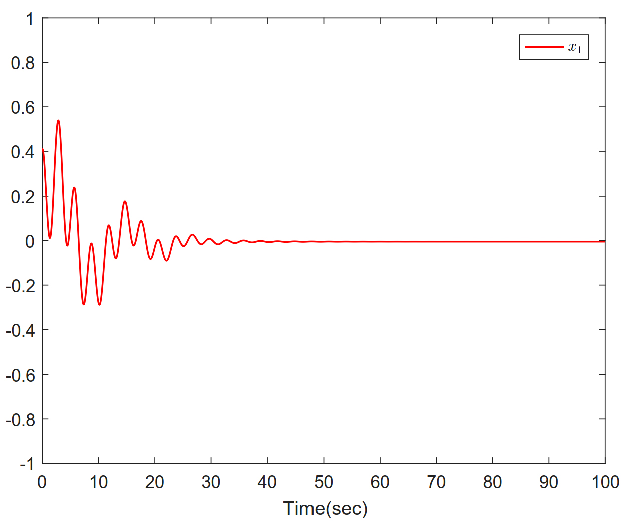
The simulation results are given as follows. Figure 1 represents the response of the state $$ x_1 $$. The response of the state $$ x_2 $$ is shown by Figure 2. Figure 3 shows the trajectories of the state $$ x_3 $$. The trajectory of the state $$ \dot{x}_1 $$ is plotted in Figure 4. Figure 5 portrays the response of the state $$ \dot{x}_2 $$. Figure 6 shows the trajectory of the input $$ u $$. The trigger time intervals are illustrated in Figure 7. The trajectories of adaptive laws are given in Figure 8, Figure 9, and Figure 10.

Adaptive backstepping control of high-order fully actuated nonlinear systems with event-triggered strategy

Figure 1. Trajectories of $$ x_1 $$ in Example 1.

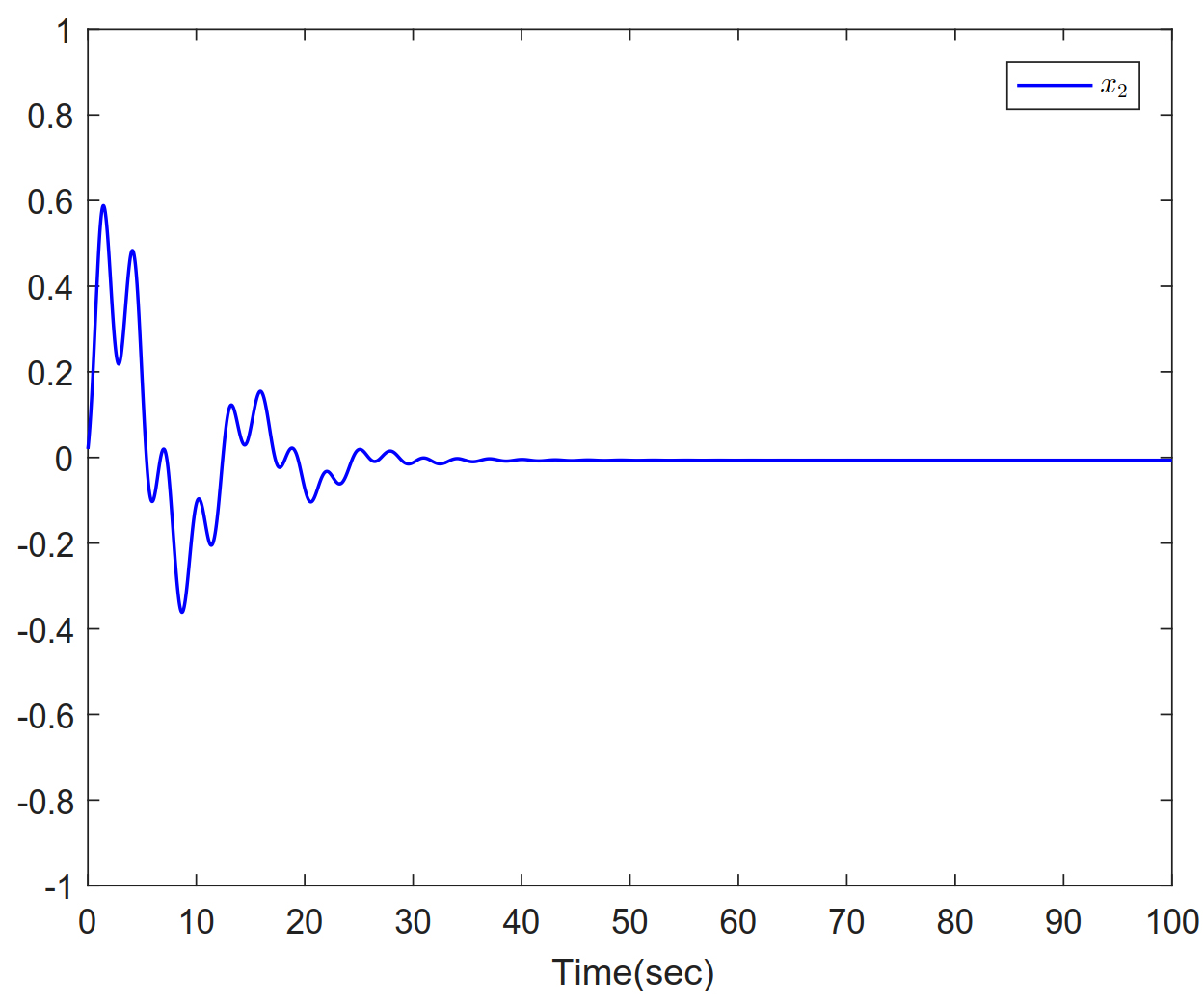
Figure 2. Trajectories of $$ x_2 $$ in Example 1.

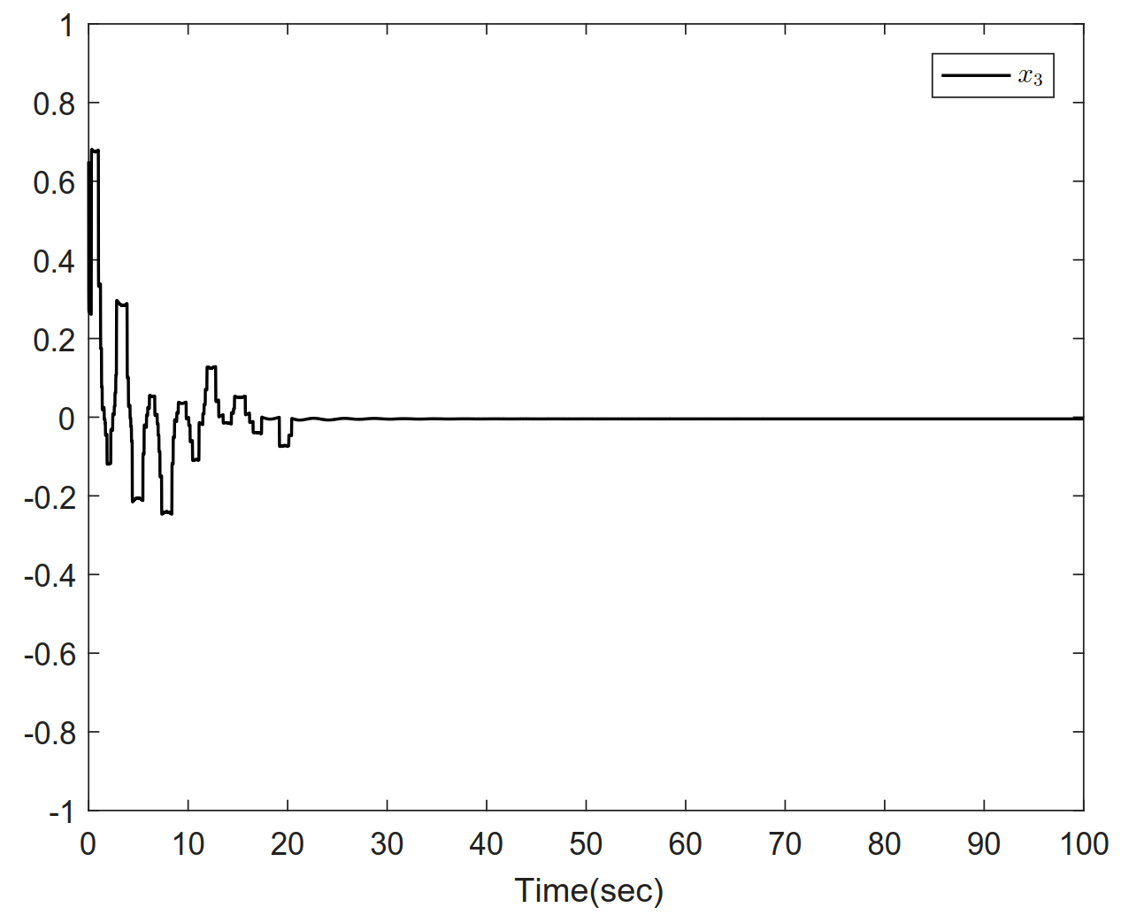
Figure 3. Trajectories of $$ x_3 $$ in Example 1.

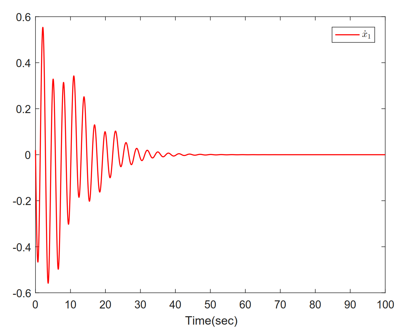
Figure 4. Trajectories of $$ \dot{x}_1 $$ in Example 1.

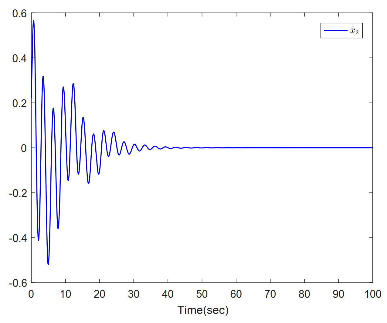
Figure 5. Trajectories of $$ \dot{x}_2 $$ in Example1.

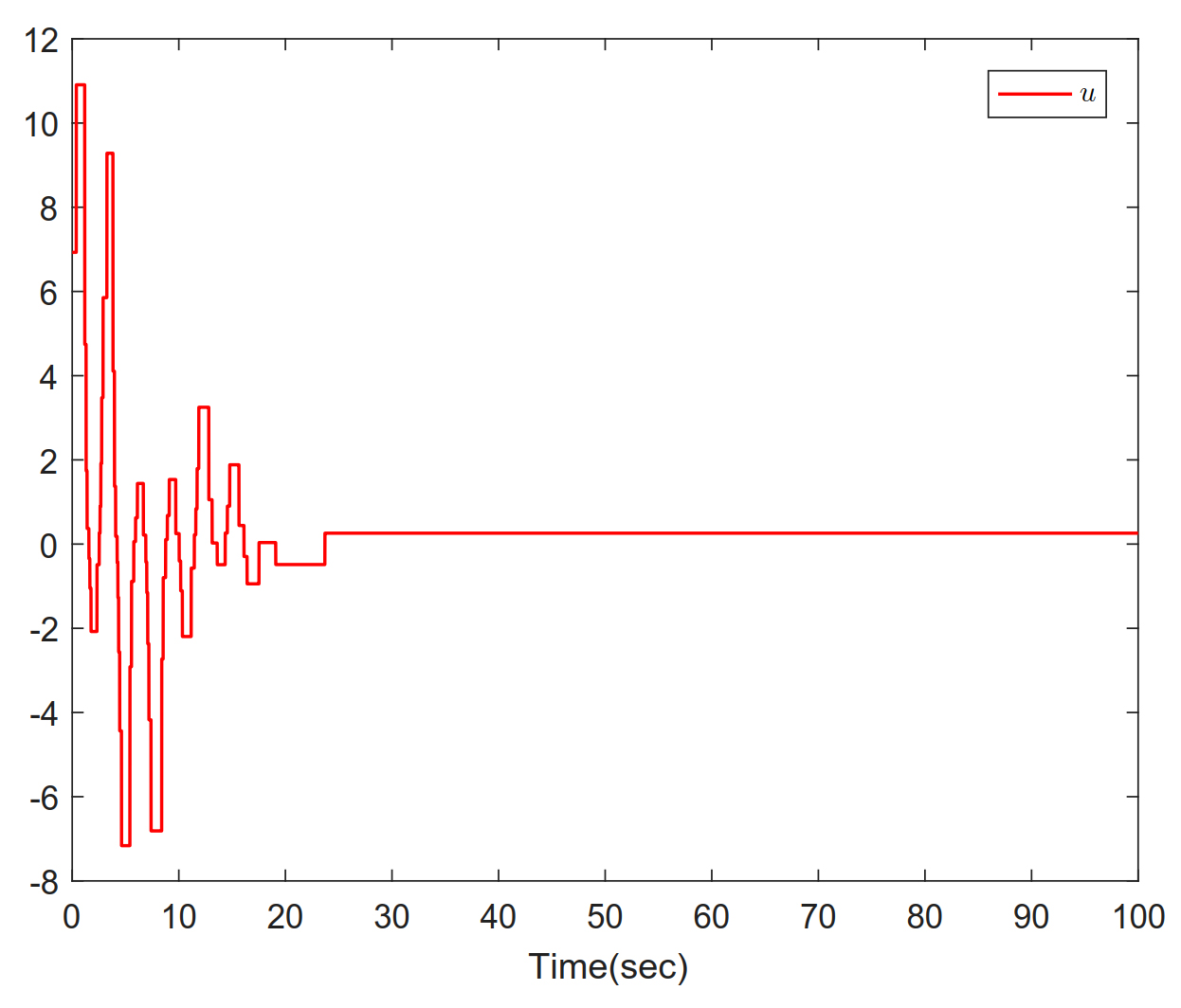
Figure 6. Trajectories of $$ u $$ in Example 1.

Figure 7. Inter-event times in Example 1.

Figure 8. Trajectories of adaptive laws $$ \hat{\theta}_1 $$ in Example 1.

Figure 9. Trajectories of adaptive laws $$ \hat{\theta}_2 $$ in Example 1.

Figure 10. Trajectories of adaptive laws $$ \hat{\theta}_3 $$ in Example 1.

5. CONCLUSIONS

In this article, a novel adaptive high-order event-triggered control scheme is proposed for uncertain HOFA nonlinear systems. This scheme not only does not require prior knowledge of the nonlinear function of the system but also saves communication resources by designing the event-triggered scheme. Moreover, the practicality of the control scheme is verified. The future of work will be concerned with the prescribed performance control problem and network attack problem of high-order fully activated nonlinear systems.

DECLARATIONS

Authors' contributions

Made substantial contributions to the conception and design of the study and performed data analysis and interpretation: Yan C, Xia J, Liu X, Yue H

Performed data acquisition and provided administrative, technical, and material support: Xia J, Li C

Availability of data and materials

Not applicable.

Financial support and sponsorship

This work was supported by the National Natural Science Foundation of China under Grants 61973148 and Discipline with Strong Characteristics of Liaocheng University: Intelligent Science and Technology under Grant 319462208.

Conflicts of interest

All authors declared that there are no conflicts of interest.

Ethical approval and consent to participate

Not applicable.

Consent for publication

Not applicable.

Copyright

REFERENCES

1. Yuan S, Lv M, Baldi M, Zhang L. Lyapunov-Equation-Based stability analysis for switched linear systems and its application to switched adaptive control. IEEE Trans Automat Contr 2021;66:2250-6.

2. Shi Y, Sun X. Bumpless transfer control for switched linear systems and its application to Aero-Engines. IEEE Trans Circuits Syst Ⅰ 2021;68:2171-82.

3. Zhang K, Zhou B, Jiang H, Liu G, Duan G. Practical prescribed-time sampled-data control of linear systems with applications to the air-bearing testbed. IEEE Trans Ind Electron 2022;69:6152-61.

4. Zhang J, Shao X, Zhang W. Cooperative enclosing control with modified guaranteed performance and aperiodic communication for unmanned vehicles: a path-following solution. IEEE Trans Ind 2023:1-10.

5. Zuo Z, Liu C, Han Q, Song J. Unmanned aerial vehicles: control methods and future challenges. IEEE/CAA J Autom Sinica 2022;9:601-14.

6. Liu Y, Zhan W, Xing M, Wu Y, Xu R, Wu X. Boundary control of a rotating and length-varying flexible robotic manipulator system. IEEE Trans Syst Man Cybern Syst 2022;52:377-86.

7. Hou Z, Xiong S. On model-free adaptive control and its stability analysis. IEEE Trans Automat Contr 2019;64:4555-69.

8. Wen G, Chen C, Ge S. Simplified optimized backstepping control for a class of nonlinear strict-feedback systems with unknown dynamic functions. IEEE Trans Cybern 2021;51:4567-80.

9. Fei J, Wang H, Fang Y. Novel neural network fractional-order sliding-mode control with application to active power filter. IEEE Trans Syst Man Cybern, Syst 2022;52:3508-18.

10. Li X, He J, Wen C, Liu X. Backstepping-Based adaptive control of a class of uncertain incommensurate fractional-order nonlinear systems with external disturbance. IEEE Trans Ind Electron 2022;69:4087-95.

11. Li Y, Hou Z, Che W, Wu Z. Event-Based design of finite-time adaptive control of uncertain nonlinear systems. IEEE Trans Neural Netw Learn Syst 2022;33:3804-13.

12. Ma J, Park J, Xu S. Command-Filter-Based finite-time adaptive control for nonlinear systems with quantized input. IEEE Trans Automat Contr 2021;66:2339-44.

13. Huang J, Wang W, Zhou J. Adaptive control design for underactuated cranes with guaranteed transient performance: theoretical design and experimental verification. IEEE Trans Ind Electron 2022;69:2822-32.

14. Lai G, Tao G, Zhang Y, Liu Z. Adaptive control of noncanonical neural-network nonlinear systems with unknown input dead-zone characteristics. IEEE Trans Neural Netw Learn Syst 2020;31:3346-60.

15. Duan G. High-order fully actuated system approaches: Part Ⅰ. Models and basic procedure. Int J Syst Sci 2021;52:422-35.

16. Duan G. High-order fully actuated system approaches: Part Ⅱ. Generalized strict-feedback systems. Int J Syst Sci 2021;52:437-54.

17. Duan G. High-order fully actuated system approaches: Part Ⅲ. Robust control and high-order backstepping. Int J Syst Sci 2021;52:952-71.

18. Duan G. High-order fully actuated system approaches: Part Ⅳ. Adaptive control and high-order backstepping. Int J Syst Sci 2021;52:972-89.

19. Duan G. High-order fully actuated system approaches: Part Ⅴ. Robust adaptive control. Int J Syst Sci 2021;52:2129-43.

20. Liu W, Duan G, Hou M. Concurrent learning adaptive command filtered backstepping control for high-order strict-feedback systems. IEEE Trans Circuits Syst Ⅰ 2023;70:1696-709.

21. Lu S, Tsakalis K, Chen Y. Development and application of a novel high-order fully actuated system approach-part Ⅰ: 3-DOF quadrotor control. IEEE Control Syst Lett 2023;7:1177-82.

22. Zhang D, Liu G, Cao L. Constrained cooperative control for high-order fully actuated multiagent systems with application to air-bearing spacecraft simulators. IEEE/ASME Trans Mechatron ; doi: 10.1109/10.1109/tmech.2022.3223927.

23. Zhang D, Liu G, Cao L. Proportional integral predictive control of high-order fully actuated networked multiagent systems with communication delays. IEEE Trans Syst Man Cybern Syst 2023;53:801-12.

24. Lian Z, Shi P, Lim C, Yuan X. Fuzzy-Model-Based lateral control for networked autonomous vehicle systems under hybrid cyber-attacks. IEEE Trans Cybern 2023;53:2600-9.

25. Pan Y, Wu Y, Lam H. Security-Based Fuzzy control for nonlinear networked control systems with dos attacks via a resilient event-triggered scheme. IEEE Trans Fuzzy Syst 2022;30:4359-68.

26. Zhang X, Han Q, Ge X, et al. Networked control systems: a survey of trends and techniques. IEEE/CAA J Autom Sinica 2020;7:1-17.

27. Jiang B, Karimi H, Kao Y, Gao C. Takagi-Sugeno model based event-triggered fuzzy sliding-mode control of networked control systems with semi-markovian switchings. IEEE Trans Fuzzy Syst 2020;28:673-83.

28. Peng C, Sun H. Switching-Like event-triggered control for networked control systems under malicious denial of service attacks. IEEE Trans Automat Contr 2020;65:3943-9.

29. Wang J, Yang C, Xia J, Wu Z, Shen H. Observer-Based sliding mode control for networked fuzzy singularly perturbed systems under weighted try-once-discard protocol. IEEE Trans Fuzzy Syst 2022;30:1889-99.

30. Chen G, Sun J, Chen J. Passivity-Based robust sampled-data control for markovian jump systems. IEEE Trans Syst Man Cybern Syst 2020;50:2671-84.

31. Chen G, Xia J, Park J, Shen H, Zhuang G. Sampled-Data synchronization of stochastic markovian jump neural networks with time-varying delay. IEEE Trans Neural Netw Learn Syst 2022;33:3829-41.

32. Xia J, Chen G, Park J, Shen H, Zhuang G. Dissipativity-Based sampled-data control for fuzzy switched markovian jump systems. IEEE Trans Fuzzy Syst 2021;29:1325-39.

33. Zou Y, Zuo Z, Xia K, Basin M. Saturated Sampled-data distributed control for interval consensus of multi-agent systems. IEEE Trans on Signal and Inf Process over Networks 2022;8:1024-36.

34. Huang J, Wang W, Wen C, Li G. Adaptive event-triggered control of nonlinear systems with controller and parameter estimator triggering. IEEE Trans Automat Contr 2020;65:318-24.

35. Zhang J, Li S, Xiang Z. Adaptive fuzzy output feedback event-triggered control for a class of switched nonlinear systems with sensor failures. IEEE Trans Circuits Syst Ⅰ 2020;67:5336-46.

36. Zhang J, Li S, Xiang Z. Adaptive event-triggered control of uncertain nonlinear systems using intermittent output only. IEEE Trans Automat Contr 2022;67:4218-25.

37. Wang X, Xia J, Park J, Xie X, Chen G. Intelligent control of performance constrained switched nonlinear systems with random noises and its application: an event-driven approach. IEEE Trans Circuits Syst Ⅰ 2022;69:3736-47.

38. Wang X, Xia J, Park J, Xie X, Chen G. Event-Triggered adaptive tracking with guaranteed transient performance for switched nonlinear systems under asynchronous switching. IEEE Trans Cybern 2023; doi: 10.1109/tcyb.2022.3223983.

39. Meng R, Hua C, Li K, Ning P. A multifilters approach to adaptive event-triggered control of uncertain nonlinear systems with global output constraint. IEEE Trans Cybern 2023; doi: 10.1109/tcyb.2022.3190861.

40. Meng R, Hua C, Li K, Ning P. Adaptive event-triggered control for uncertain high-order fully actuated system. IEEE Trans Circuits Syst Ⅱ 2022;69:4438-42.

41. Yang D, Zong G, Su S. H∞ Tracking control of uncertain markovian hybrid switching systems: a fuzzy switching dynamic adaptive control approach. IEEE Trans Cybern 2020;52:3111-22.

42. Chen H, Zong G, Gao F, Shi Y. Probabilistic event-triggered policy for extended dissipative finite-time control of mjss under cyber-attacks and actuator failures. IEEE Trans Automat Contr 2023; doi: 10.1109/tac.2023.3246429.

43. Chen H, Zong G, Zhao X, Gao F, Shi K. Secure filter design of fuzzy switched cpss with mismatched modes and application: a multidomain event-triggered strategy. IEEE Trans Ind Inf 2022; doi: 10.1109/tii.2022.3232768.

Cite This Article

Export citation file: BibTeX | RIS

OAE Style

Yan C, Xia J, Liu X, Yue H, Li C. Adaptive backstepping control of high-order fully actuated nonlinear systems with event-triggered strategy. Intell Robot 2023;3(2):176-89. http://dx.doi.org/10.20517/ir.2023.11

AMA Style

Yan C, Xia J, Liu X, Yue H, Li C. Adaptive backstepping control of high-order fully actuated nonlinear systems with event-triggered strategy. Intelligence & Robotics. 2023; 3(2): 176-89. http://dx.doi.org/10.20517/ir.2023.11

Chicago/Turabian Style

Yan, Chengyuan, Jianwei Xia, Xinru Liu, Huarong Yue, Chong Li. 2023. "Adaptive backstepping control of high-order fully actuated nonlinear systems with event-triggered strategy" Intelligence & Robotics. 3, no.2: 176-89. http://dx.doi.org/10.20517/ir.2023.11

ACS Style

Yan, C.; Xia J.; Liu X.; Yue H.; Li C. Adaptive backstepping control of high-order fully actuated nonlinear systems with event-triggered strategy. Intell. Robot. 2023, 3, 176-89. http://dx.doi.org/10.20517/ir.2023.11

About This Article

Special Issue

This article belongs to the Special Issue Robot System Intelligentization and Application: Learning, Control and Decision

Copyright

© The Author(s) 2023. Open Access This article is licensed under a Creative Commons Attribution 4.0 International License (https://creativecommons.org/licenses/by/4.0/), which permits unrestricted use, sharing, adaptation, distribution and reproduction in any medium or format, for any purpose, even commercially, as long as you give appropriate credit to the original author(s) and the source, provide a link to the Creative Commons license, and indicate if changes were made.

Data & Comments

Data

Views

427

Downloads

Citations

Comments

Comments

Comments must be written in English. Spam, offensive content, impersonation, and private information will not be permitted. If any comment is reported and identified as inappropriate content by OAE staff, the comment will be removed without notice. If you have any queries or need any help, please contact us at support@oaepublish.com.